Two-Level Factors: The 2 k Factorial Design When several factors may - PowerPoint PPT Presentation

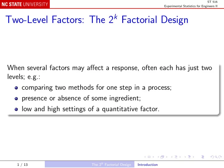
ST 516 Experimental Statistics for Engineers II Two-Level Factors: The 2 k Factorial Design When several factors may affect a response, often each has just two levels; e.g.: comparing two methods for one step in a process; presence or absence of some ingredient; low and high settings of a quantitative factor. The 2 k Factorial Design 1 / 13 Introduction

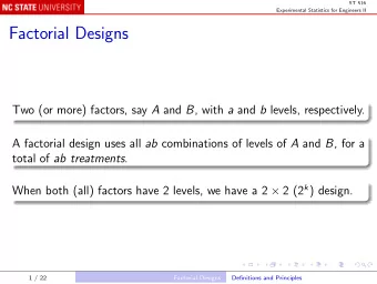
ST 516 Experimental Statistics for Engineers II k factors, each with 2 levels, give 2 k treatment combinations. The 2 k (full, or complete) factorial design uses all 2 k treatments. It requires the fewest runs of any factorial design for k factors. Often used at an early stage: factor screening experiments. The 2 k Factorial Design 2 / 13 Introduction

ST 516 Experimental Statistics for Engineers II The 2 2 Design Notation Factors are usually A , B , etc. The two levels of each are usually denoted “+” and “-”. E.g. 2 2 : Factor Treatment Treatment Total of A B Combination Label Responses - - A low, B low (1) (1) + - A high, B low a a - + A low, B high b b + + A high, B high ab ab The 2 k Factorial Design The 2 2 Design 3 / 13

ST 516 Experimental Statistics for Engineers II Hand calculation of effects Simple effect of A at low level of B is difference between average n − (1) responses: a n , where n = number of replicates. Simple effect of A at high level of B is difference between average responses: ab n − b n . Main effect of A (also denoted A ) is the average of these: A = 1 2 n [ ab + a − b − (1)] The 2 k Factorial Design The 2 2 Design 4 / 13

ST 516 Experimental Statistics for Engineers II Similarly main effect of B is B = 1 2 n [ ab + b − a − (1)] The interaction effect AB is one half of the difference between: the simple effect of A at the high level of B ; and the simple effect of A at the low level of B : AB = 1 2 n [ ab + (1) − a − b ] AB is also (one half of) the difference between the effects of B at the two levels of A . The 2 k Factorial Design The 2 2 Design 5 / 13

ST 516 Experimental Statistics for Engineers II Example: 2 2 with 3 replications Factors: A = reactant concentration, levels 15% and 25%; B = catalyst, levels 1lb and 2lb. Response: yield. The 2 k Factorial Design The 2 2 Design 6 / 13

ST 516 Experimental Statistics for Engineers II Data: (yield.txt) A B Rep Yield - - I 28 + - I 36 - + I 18 + + I 31 - - II 25 + - II 32 - + II 19 + + II 30 - - III 27 + - III 32 - + III 23 + + III 29 Note The runs are listed in the “standard” order; in a CRD, they would be carried out in a random order. The 2 k Factorial Design The 2 2 Design 7 / 13

ST 516 Experimental Statistics for Engineers II R Analysis of Variance yield <- read.table("data/yield.txt", header = TRUE) par(mfrow = c(1, 2)) plot(Yield ~ A * B, yield) par(mfrow = c(1, 1)) with(yield, interaction.plot(A, B, Yield)) summary(aov(Yield ~ A * B, yield)) plot(aov(Yield ~ A * B, yield)); # the usual suspects Output Df Sum Sq Mean Sq F value Pr(>F) A 1 208.333 208.333 53.1915 8.444e-05 *** B 1 75.000 75.000 19.1489 0.002362 ** A:B 1 8.333 8.333 2.1277 0.182776 Residuals 8 31.333 3.917 --- Signif. codes: 0 *** 0.001 ** 0.01 * 0.05 . 0.1 1 The 2 k Factorial Design The 2 2 Design 8 / 13

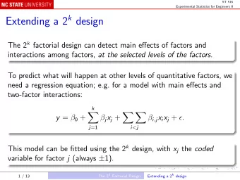
ST 516 Experimental Statistics for Engineers II Effects Fit the regression equation, with versions of the factors coded as − 1 for low levels of each, and +1 for high levels: coded <- function(x) ifelse(x == x[1], -1, 1) summary(lm(Yield ~ coded(A) * coded(B), yield)) The 2 k Factorial Design The 2 2 Design 9 / 13

ST 516 Experimental Statistics for Engineers II Output Call: lm(formula = Yield ~ coded(A) * coded(B), data = yield) Residuals: Min 1Q Median 3Q Max -2.000 -1.333 -0.500 1.083 3.000 Coefficients: Estimate Std. Error t value Pr(>|t|) (Intercept) 27.5000 0.5713 48.135 3.84e-11 *** coded(A) 4.1667 0.5713 7.293 8.44e-05 *** coded(B) -2.5000 0.5713 -4.376 0.00236 ** coded(A):coded(B) 0.8333 0.5713 1.459 0.18278 --- Signif. codes: 0 *** 0.001 ** 0.01 * 0.05 . 0.1 1 Residual standard error: 1.979 on 8 degrees of freedom Multiple R-Squared: 0.903, Adjusted R-squared: 0.8666 F-statistic: 24.82 on 3 and 8 DF, p-value: 0.0002093 The 2 k Factorial Design The 2 2 Design 10 / 13

ST 516 Experimental Statistics for Engineers II Note A coefficient in a regression equation is the change in the response when the corresponding variable changes by +1. As A or B changes from its low level to its high level, the coded variable changes by 1 − ( − 1) = +2, so the change in the response is twice the regression coefficient. So the effects and interaction(s) are twice the values in the “Estimate” column. These regression coefficients are often called effects and interactions, even though they differ from the definitions given earlier. The 2 k Factorial Design The 2 2 Design 11 / 13

ST 516 Experimental Statistics for Engineers II Hand calculation of effects and interactions Yates’s algorithm: Sums Intermediate Step Effects (1) (1) + a (1) + a + b + ab = 4 n ˆ µ b + ab − (1) + a − b − ab = 2 nA a b − (1) + a − (1) − a + b + ab = 2 nB − b + ab (1) − a − b + ab = 2 nAB ab Eight additions and subtractions instead of twelve! (More advantage for large k .) The 2 k Factorial Design The 2 2 Design 12 / 13

ST 516 Experimental Statistics for Engineers II Response surface When both A and B are quantitative, the regression equation can be used to predict the expected response at other values of the factors: yield <- within(yield, {cA = coded(A); cB = coded(B)}) yieldLm <- lm(Yield ~ cA * cB, data = yield) ngrid <- 20 Agrid <- Bgrid <- seq(from = -1, to = 1, length = ngrid) yhat <- predict(yieldLm, expand.grid(cA = Agrid, cB = Bgrid)) yhat <- matrix(yhat, length(Agrid), length(Bgrid)) persp(Agrid, Bgrid, yhat, theta = -40, phi = 30) # in real values: persp(20 + 5 * Agrid, 1.5 + 0.5 * Bgrid, yhat, theta = -40, phi = 30, ticktype = "d", xlab = "Reactant Concentration", ylab = "Catalyst") The 2 k Factorial Design The 2 2 Design 13 / 13