Tumor growth: From mathematical models to clinical applications - PowerPoint PPT Presentation

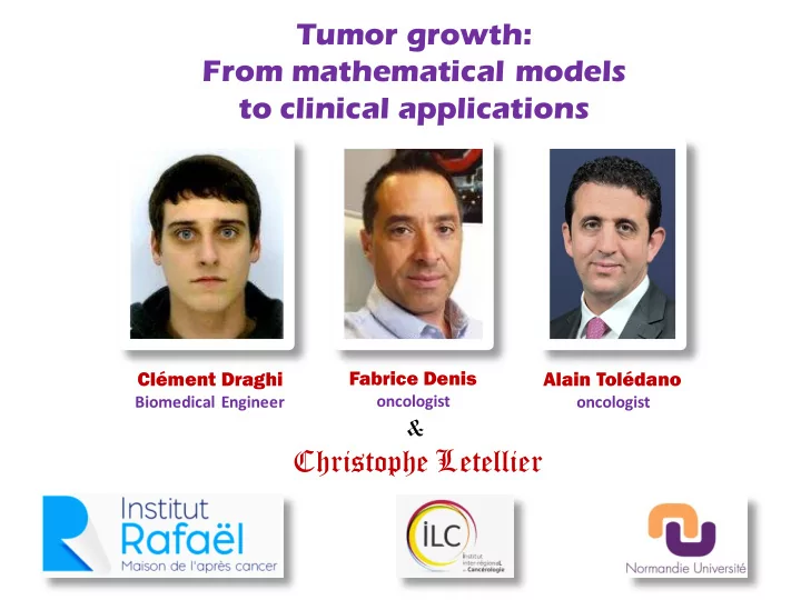
Tumor growth: From mathematical models to clinical applications Clément Draghi Fabrice Denis Alain Tolédano Biomedical Engineer oncologist oncologist & Christophe Letellier

Outline in few words  Why genetics cannot explain everything  A simple model taking into account the microenvironment  Spatial growth versus local dynamics  Cancer risk depends on the tissue  A web-mediated follow-up  A model for the PSA level in patients with prostate cancer

Incidence of cancers in US in 2014 Cancer risk strongly depends on the organ

External factors affecting cancer risk during lifetime Hereditary syndrome Obesity (genetic mutation) Lack of physical activity Alcohol Tobacco addiction addiction Bad quality food 10% Tissular dynamics State of the tissue = Cell interaction

Cancer risk : ‘’ bad luck ’’ or not? Lifetime risk of cancer of many r = 0.81, p < 4  10 -8 different types is strongly correlated with the total number of divisions of the normal self- renewing cells … The majority of the variations in cancer risk is due to bad luck , that is, random mutations arising during DNA replication in normal stem cells.

 Cancer incidence versus age Hypothesis : the probability to present tumor cells depends on the number of cell divisions during life Corollary : The longer the life, the larger the cancer risk In the United-Kingdom Evolution of life expectancy (all types of cancer included) Average number of deaths per year r man r woman N man N woman Life expectancy (year) 40 years 40 years year Age at death  The probability does not increase linearly with age …

Peto’s paradox Hypothesis: The probability to observe a malign cell depends on the number of cell divisions during the lifetime Corollary: bowhead whale should present much more cancers than humans …  They frequently survive up to 250 years without cancer!  Their immune system is 4 times more efficient!

Role of the microenvironment Hypothesis: the probability to present malign cells depends on the number of cell divisions during the lifetime but detecting a tumour depends more on the barriers developed by the microenvironment Corollary 3: the probability to initiate a cancer depends more on the state of the microenvironment than on the presence of malign cells Modification of the microenvironment

A cancer model Interactions between cell populations in a single tumor site + x Host cells - - - Tumor Immune y contramensalism cells cells z + - ±

Realistic parameter values? Colons x 100 5.4 3.4 391 x 65 1.2 3.4 219 Prostate Breast Skin x 26 Lung 4.1 4.4 114

 Chaotic oscillations in the cancer model Growth rate r h = 0.54 Host cells Tumor cells Prostate Specific Antigen PSA (ng/ml) Time (days)

 Very agressive cancers can also be observed A clinical example Growth rate r h =1.45 Host cells Tumor cells 14 days later …. Man, 67 years Smoker Pulmonary adenocarcinoma

 Role of immune cells Influence of the inhibition of tumor cells by immune cells Tumor cells The action of immune cells does not affect the dynamics Inhibition rate r ti of tumor cells by immune cells  Sometimes immunotherapy is of a limited interest … anti PD-1 (Nivolumab) immunotherapy 3 month later …. Woman, 64 years Smoker Adenocarcinoma with bone metastases

Spatial simulations of tumor growth  Depends on the inhibition of immune cells by tumor cells 𝛽 IT = 3.0 𝛽 IT = 1.9  T ≈ 2.9 mm  T ≈ 1.3 mm In the lung of a woman After 6000 a.u.t. 64 years, smoker, adenocarcinoma with a bone metastasis Immune cells Immune cells Proliferation Local dynamics Quiescence (proliferation) Necrosis Tumor cells Tumor cells

Spatial simulations of tumor growth  The tumor growth depends on the inhibition of immune cells by tumor cells After Dynamics 74 800 a.u.t. in each site Proliferation 𝛽 IT = 0,3015 Immune cells r I = 5,05 Quiescence D ≈ 1.7 mm Necrosis Tumor cells  Chaotic dynamics in each site  Very few sites have tumor cells  Very slow tumor growth

Spatial simulations of tumor growth  When the local dynamics is chaotic t = 74 800 a.u.t. Local dynamics  Heterogeneous Immune cells  Proliferation zone is thick  Slow tumor growth Tumor cells  Woman, 80 years, smoker up to 60 years: weakly evolutive nodule 6 March 2014 6 July 2015 Adenocarcinoma

 Dynamics more important than cell interaction  Equivalent dynamics but different parameter values ρ H = 0.4862 ρ H = 0.5015 ρ H = 0.5015 ρ I = 5.05 ρ I = 5.007 ρ I = 5.119 α IT = 0.3015 α IT = 0.504 α IT = 0.624 𝐸 ≈ 1.1 mm 𝐸 ≈ 1.1 mm 𝐸 ≈ 1.7 mm  With equivalent dynamics, the role of the microenvironment is relevant  The growth rate of host cells is a very influent parameter …

How depends cancer risk on the tissue?  Our hypotheses  The nature of tissue is distinguished by the growth rate r H of host cells  The growth rate r T of tumor cells in a given tissue is twice the growth rate of host cells ( r T = 2 r H )  The quality of the tissue (How strong are the barriers againt tumor growth) depends on other parameters (which can be affected by external factors)  Varying parameter values = creation of a cohort of patients randomly chosen

 How can cancer risk depend on normal cells?  The probability to detect a tumor depends on the growth rate of host cells, that is, on how competitive are the normal cells Probability P for a tumor Host cell growth rate r H

 E volution of a cancer… Do we observe this correctly? Do we measure the right variable?  There is a mathematical background for addressing this question…  Observability (from control theory)

 The observability matrix Original state space - f ( x ) : R m  R m is the dynamical system 𝒚 = 𝒈 𝒚 𝑡 𝑢 = ℎ 𝒚 where - h ( x ) : R m  R is the measurement function Between the original and the reconstructed spaces, the change of coordinates 0 ℎ 𝒚 = 𝑡 𝑢 𝑌 = 𝑀 𝑔  1    j L h x 1 ℎ 𝒚 = 𝑡 𝑢     𝑍 = 𝑀 𝑔 f Φ = where  j L are Lie derivatives h x f x f  x 2 ℎ 𝒚 = 𝑡 𝑢 𝑎 = 𝑀 𝑔 Observability matrix 0 ℎ 𝒚 𝜖𝑀 𝒈 The system f ( x ) is said to be observable if 𝜖𝒚 the observability matrix is full rank. 𝑃 𝑡 𝒚 = ⋮  Full observability 𝑛−1 ℎ 𝒚 𝜖𝑀 𝒈 𝜖𝒚  every states x i and x j are distinguishable with respect to the measured variable s ( t ), that is, h ( x i )  h ( x j ) iff x i  x j

 Conditions for a full observability Original state space Reconstructed space (Rössler system) Coordinate transformation 𝑌 = 𝑧 𝑦 = −𝑧 − 𝑨 𝑌 = 𝑍 Z 𝑍 = 𝑧 = 𝑦 + 𝑏𝑧 z Φ 𝑧 = 𝑧 = 𝑦 + 𝑏𝑧 𝑍 = 𝑎 𝑎 = 𝑧 = 𝑏𝑦 + 𝑏 2 − 1 𝑧 − 𝑨 𝑨 = 𝑐 + 𝑦 − 𝑑 𝑎 = 𝐺 𝑌, 𝑍, 𝑎 𝒆 = 𝟒 𝒆 𝒔 = 𝟒 Diffeomorphism if Det J F  0 y x Y X   0 1 0     Det J Det 1 a 0 1   F y     2 a a 1 1   The Rössler system is fully observable from variable y(t)  Jacobian matrix of Φ 𝑧 ≝ 𝐩𝐜𝐭𝐟𝐬𝐰𝐛𝐜𝐣𝐦𝐣𝐮𝐳 𝐧𝐛𝐮𝐬𝐣𝐲

 Singular observability manifold  Definition of the neighborhood of the singular observability manifold from the determinant of 𝐾 𝛸 𝑦 ∉ 𝐵 ∩ 𝑉 𝑁 𝑡  Assessing the probability for 𝑝𝑐𝑡 𝑁 = 1.00 𝜃 𝑧

 Observability of the cancer model > > The worse! The best! Tumor cells Immune cells Hot cells It should be more efficient to follow the tumor environment than the tumor itself!

 Application to lung cancer Non smoking Smoking

 Web-mediated follow-up: weekly self-evaluated symptoms  rationale : since host cells provides a better observability of the dynamic, could we follow the 1. Weight environment rather than the tumor itself? 2. Apetite loss 3. Weakness 4. Pain Environment = global patient’s state 5. Cough weekly self-evaluated 6. Breathlessness  A cohort of 121 patients treated for a lung cancer 1. Pulmonary carcinome (stade 3-4) 2. Web access

 Web-mediated follow-up: weekly self-evaluated symptoms

 Web-mediated follow-up: weekly self-evaluated symptoms Man, 63 years  Patient without relapse Smoker, 90 kg, no exercise Treated by radiotherapy Relapse probability = 75 % August 9 November 23 Before radiotherapy

 Web-mediated follow-up: weekly self-evaluated symptoms Man, 65 years  Patient with relapse Smoker, 86 kg, no exercise Treated by chemiotherapy Relapse probability = 75 % August 19 January 6  2 months before the routine imaging

 Web-mediated follow-up: weekly self-evaluated symptoms Confusion matrix With Without relapse relapse Other diseases Breathlessness Moovcare positive 13 3 Moovcare negative 0 25 Sensibility 100% 85% Specificity 89% 96%  Detecting cancer relapse five weeks earlier than using routine imagings !  Reliability equivalent to a classical follow-up!