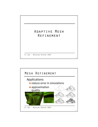
Towards achieving GPU-native adaptive mesh refinement Ania Brown - PowerPoint PPT Presentation

Towards achieving GPU-native adaptive mesh refinement Ania Brown Prof Takayuki Aoki

Why AMR?


 AMR is not GPU friendly • Complicated, time varying data structures • Can you use AMR and keep GPU performance? 
 My conclusion: yes, but it’s messy

Contents • Introduction to the algorithm + data structures • The challenges • Optimisation possibilities • The RSE perspective — some lessons learnt

Problem domain i, j+1 • Stencil calculations on a i-1, j i, j i+1, j square structured mesh i, j-1 • Cell centre values

1) Block structured AMR

1) Block structured AMR

1) Block structured AMR

2) Tree based AMR Simulation mesh Refinement representation

2) Tree based AMR Simulation mesh Refinement representation

2) Tree based AMR Simulation mesh Refinement representation

2) Tree based AMR Simulation mesh Refinement representation … …

2) Tree based AMR Simulation mesh Refinement representation … … … …

3) Patches +Tree AMR

CPU GPU Block-structured Octree + patches GAMER (2011) Enzo Daino (2016) CHOMBO Octree RAMSES Octree + patches FLASH, using PARAMESH NIRVANA

The AMR algorithm Initialize data structures Main loop: Create halo regions Update patch values Refine/coarsen patches Update neighbour relations Output values for visualisation

CPU GPU Initialize data structures Main loop: Create halo regions Update patch values Refine/coarsen patches Update neighbour relations Output values for visualisation

Update step 1 CUDA block

Update step • Tune block size for coalesced access • Zmarching

CPU GPU Initialize data structures Main loop: Create halo regions Update patch values Refine/coarsen patches Update neighbour relations Output values for visualisation

CPU GPU Initialize data structures Main loop: Create halo regions Update patch values Refine/coarsen patches Update neighbour relations Output values for visualisation

Ordering leaves

Hilbert curve At each step: • Divide space into 4 • Replace each quadrant with rotated or reflected versions of the original curve • Connect such that that start and end points remain the same

Rules for refinement

Neighbour relations Leaf nodes: 
 Neighbour indices in each direction Parent index Parent nodes: Child indices

Create halo regions Find correct neighbour node

Create halo regions Find correct neighbour node

Create halo regions Find correct neighbour node

Create halo regions Copy halo values

Interpolating halo values

Interpolating halo values

Interpolating halo values

Interpolating halo values

Interpolating halo values

Reducing halo values

Reducing halo values

Coarsen/refine step CPU GPU Main loop: Find patches to coarsen/refine Refine/coarsen patch values Update neighbour relations Defragment value array

Defragment value array refine node

Defragment value array refine node

Defragment value array refine node

Defragment value array coarsen node

Defragment value array coarsen node

Defragment value array coarsen node

Calculate new defragmented position • Input: for all nodes, flag whether that node is to be refined, coarsened or unchanged • Refined: +3 
 Coarsened: -3 
 Unchanged: 0 • For each element, sum all preceding elements in the array • For n nodes, requires n/2 threads and O(log2(n)) serial steps

Multi-GPU Load balancing

Boundaries between subdomains

Boundaries between subdomains Node 0 Node 2 Node 1

Boundaries between subdomains Node 0 Node 2 Node 1

How to distribute tree

How to distribute tree

Software design • Code framework — allow user to edit/add functions for initialisation, resolution criterion, stencil calc • Code generation — annotated regular data structures • How much to offer? — cell/node centre, interpolation level, stencil type

Software development process • Unit testing • Verification • Profiling

Phase field model of dendritic solidification in a binary alloy Code by: T.Shimokawabe, T.Takaki (2011)

7 refinement levels in quad-tree

Regular mesh Adaptive mesh

Performance testing for dendritic solidification model L = 1 . 5 × 10 − 3 m R = 4 . 5 × 10 − 4 m ∆ x min = 6 × 10 − 6 m ∆ x max = 1 . 2 × 10 − 5 m 256 x 256

Performance testing for dendritic solidification model L = 1 . 5 × 10 − 3 m R = 4 . 5 × 10 − 4 m ∆ x min = 1 . 9 × 10 − 7 m ∆ x max = 1 . 2 × 10 − 5 m 8192 x 8192

AMR Regular Mesh Worst case AMR 250 Execution time per timestep (ms) 187.5 125 62.5 0 1 2 3 4 5 6 7 8 5 2 0 0 0 0 1 1 1 1 1 5 2 4 7 9 2 4 6 9 2 6 4 8 2 6 0 4 8 2 Resolution

In summary • Patch based tree-AMR • For quick gains, offload update step to GPU • GPU-native version possible — values on GPU, neighbour relations on CPU • Likely won’t be a one size fits all fix

Governing PDEs for phase field model Diffusion Interface anisotropy  ∂φ r · ( a 2 r φ ) + ∂ ∂ x ( a ∂ a | r φ | 2 ) + ∂ ∂ y ( a ∂ a | r φ | 2 ) = � M φ ∂ t ∂φ x ∂φ y Chemical driving force Phase change � | r φ | 2 ) � S ∆ T dp ( φ ) � W dq ( φ ) + ∂ ∂ z ( a ∂ a ∂φ z d φ d φ ∂ c ∂ t = r · [ D S φ r c S + D L (1 � φ ) r c L ] : mobility M φ : interface anisotropy φ ( x, y, t ) a : phase p ( φ ) , q : interpolating function c ( x, y, t ) c = (1 − φ ) c L + φ c S q ( φ ) : double well function : diffusion in solid, liquid : liquid concentration D S , D L c L : entropy of fusion : solid concentration S c S : height of double well potential W : temperature T