Todays Outline Reinforcement Learning II Dan Weld Review - PDF document
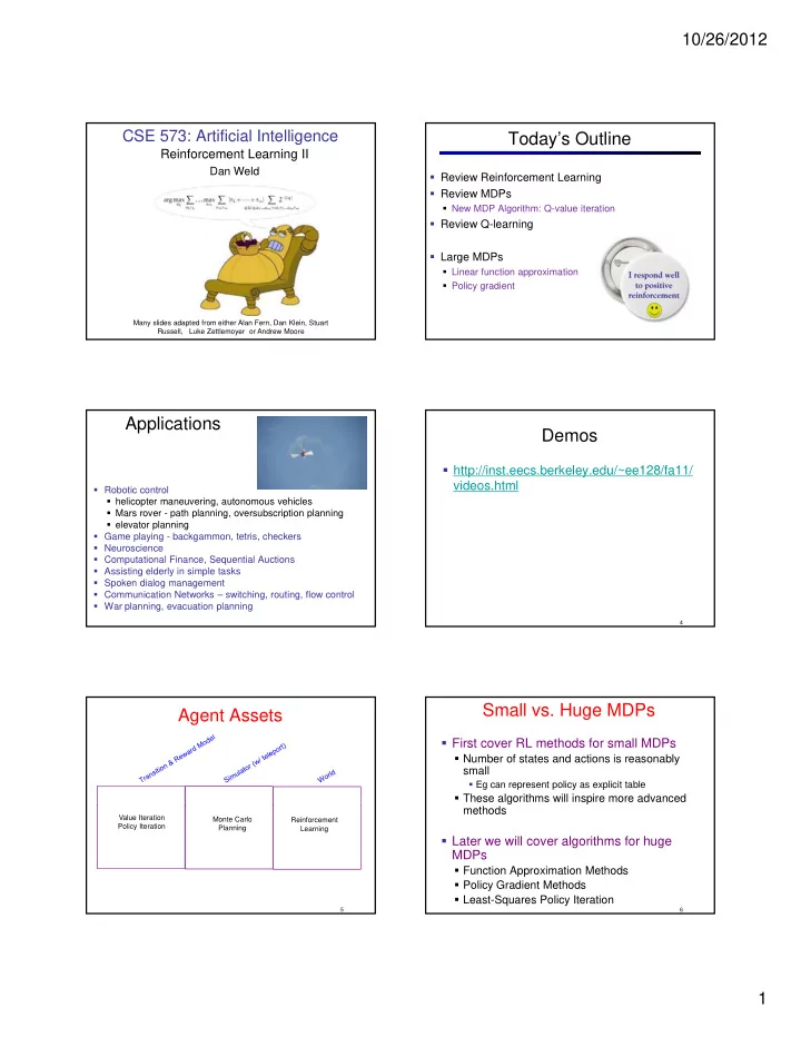
10/26/2012 CSE 573: Artificial Intelligence Todays Outline Reinforcement Learning II Dan Weld Review Reinforcement Learning Review MDPs New MDP Algorithm: Q-value iteration Review Q-learning Large MDPs Linear function
10/26/2012 CSE 573: Artificial Intelligence Today’s Outline Reinforcement Learning II Dan Weld Review Reinforcement Learning Review MDPs New MDP Algorithm: Q-value iteration Review Q-learning Large MDPs Linear function approximation Policy gradient Many slides adapted from either Alan Fern, Dan Klein, Stuart Russell, Luke Zettlemoyer or Andrew Moore 1 Applications Demos http://inst.eecs.berkeley.edu/~ee128/fa11/ videos.html Robotic control helicopter maneuvering, autonomous vehicles Mars rover - path planning, oversubscription planning g g elevator planning Game playing - backgammon, tetris, checkers Neuroscience Computational Finance, Sequential Auctions Assisting elderly in simple tasks Spoken dialog management Communication Networks – switching, routing, flow control War planning, evacuation planning 4 Small vs. Huge MDPs Agent Assets First cover RL methods for small MDPs Number of states and actions is reasonably small Eg can represent policy as explicit table These algorithms will inspire more advanced methods Value Iteration Monte Carlo Reinforcement Policy Iteration Planning Learning Later we will cover algorithms for huge MDPs Function Approximation Methods Policy Gradient Methods Least-Squares Policy Iteration 5 6 1
10/26/2012 Passive vs. Active learning Model-Based vs . Model-Free RL Model-based approach to RL: Passive learning learn the MDP model, or an approximation of it The agent has a fixed policy and tries to learn the utilities of states by observing the world go by use it for policy evaluation or to find the optimal Analogous to policy evaluation policy Often serves as a component of active learning algorithms Often inspires active learning algorithms Often inspires active learning algorithms Model-free approach to RL: Active learning derive optimal policy w/o explicitly learning the The agent attempts to find an optimal (or at least good) policy model by acting in the world useful when model is difficult to represent Analogous to solving the underlying MDP, but without first being given the MDP model and/or learn We will consider both types of approaches 7 8 Comparison RL Dimensions TD Learning Model-based approaches: Learn T + R Optimistic Q Learning Explore / RMax |S| 2 |A| + |S||A| parameters (40,400) ADP -greedy Active Model-free approach: ADP Learn Q TD Learning Direct Estimation |S||A| parameters (400) Passive Uses Model Model Free Supposing 100 states, 4 actions… 10 Recap: MDPs Markov decision processes: Bellman Equations s States S a Actions A s, a Transitions T(s,a,s ʼ ) aka P(s ʼ |s,a) s,a,s ʼ Rewards R(s,a,s ʼ ) (and discount ) s ʼ Start state s 0 (or distribution P 0 ) 0 ( 0 ) Algorithms Value Iteration Q-value iteration Q*(a, s) = Quantities: Policy = map from states to actions Utility = sum of discounted future rewards Q-Value = expected utility from a q-state Andrey Markov Ie. from a state/action pair (1856 ‐ 1922) 12 2
10/26/2012 Q- Value Iteration Q-Value Iteration Regular Value iteration: find successive approx optimal values Initialize each q-state: Q 0 (s,a) = 0 Start with V 0 * (s) = 0 Given V i * , calculate the values for all states for depth i+1: Repeat Q i+1 (s,a) For all q-states, s,a Compute Q i+1 (s,a) from Q i by Bellman backup at s,a. Until max s,a |Q i+1 (s,a) – Q i (s,a)| < V i (s’) ] Storing Q-values is more useful! Start with Q 0 * (s,a) = 0 Given Q i * , calculate the q-values for all q-states for depth i+1: V i (s’) ] Reinforcement Learning Recap: Sampling Expectations Markov decision processes: Want to compute an expectation weighted by P(x): States S s Actions A a Transitions T(s,a,s ʼ ) aka P(s ʼ |s,a) Rewards R(s,a,s ʼ ) (and discount ) s, a Model-based: estimate P(x) from samples, compute expectation Start state s 0 (or distribution P 0 ) s,a,s ʼ 0 ( 0 ) s ʼ Algorithms Q-value iteration Q-learning Model-free: estimate expectation directly from samples Why does this work? Because samples appear with the right frequencies! Q-Learning Update Recap: Exp. Moving Average Exponential moving average Q-Learning = sample-based Q-value iteration Makes recent samples more important How learn Q*(s,a) values? ( , ) Receive a sample (s,a,s ʼ ,r) Forgets about the past (distant past values were wrong anyway) Consider your old estimate: Easy to compute from the running average Consider your new sample estimate: Decreasing learning rate can give converging averages Incorporate the new estimate into a running average: 3
10/26/2012 Q-Learning Update Exploration / Exploitation Alternatively…. greedy difference = sample – Q(s, a) Every time step, flip a coin: with probability , act randomly Q-Learning = sample-based Q-value iteration With probability 1- , act according to current policy Exploration function How learn Q*(s,a) values? ( , ) Receive a sample (s,a,s ʼ ,r) Explore areas whose badness is not (yet) established Takes a value estimate and a count, and returns an Consider your old estimate: optimistic utility , e.g. Consider your new sample estimate: (exact form not important) Exploration policy π ( s ’ )= Incorporate the new estimate into a running average: vs. Q-Learning: Greedy Q-Learning Final Solution Q-learning produces tables of q-values: QuickTime™ and a H.264 decompressor are needed to see this picture. Q-Learning – Small Problem Q-Learning Properties Doesn’t work Amazing result: Q-learning converges to optimal policy If you explore enough If you make the learning rate small enough In realistic situations, we can’t possibly learn about … but not decrease it too quickly! every single state! Not too sensitive to how you select actions (!) y ( ) Too many states to visit them all in training Too many states to visit them all in training Too many states to hold the q-tables in memory Neat property: off-policy learning learn optimal policy without following it (some caveats) Instead, we need to generalize : Learn about a few states from experience Generalize that experience to new, similar states (Fundamental idea in machine learning) S E S E 4
10/26/2012 RL Dimensions Example: Pacman Let ʼ s say we discover through experience that this state is bad: Active In naïve Q learning, Many States we know nothing about related states and their Q values: Passive Uses Model Or even this third one! Model Free 25 Feature-Based Representations Linear Feature Functions Using a feature representation, we can write a Solution: describe a state using a vector of features (properties) q function (or value function) for any state Features are functions from states to using a linear combination of a few weights: real numbers (often 0/1) that capture important properties of the state Example features: Example features: Distance to closest ghost Advantage: our experience is summed up in Advantage: Distance to closest dot Number of ghosts a few powerful numbers 1 / (dist to dot) 2 Is Pacman in a tunnel? (0/1) |S| 2 |A| ? |S||A| ? …… etc. Disadvantage: states may share features but Disadvantage: Can also describe a q-state (s, a) with features actually be very different in value! (e.g. action moves closer to food) Function Approximation Example: Q-Pacman Q-learning with linear q-functions: Exact Q ʼ s Approximate Q ʼ s Intuitive interpretation: Adjust weights of active features E.g. if something unexpectedly bad happens, disprefer all states with that state ʼ s features Formal justification: online least squares 5
10/26/2012 Q-learning with Linear Approximators Q-learning, no features, 50 learning trials: 1. Start with initial parameter values 2. Take action a according to an explore/exploit policy (should converge to greedy policy, i.e. GLIE) transitioning from s to s’ 3. Perform TD update for each parameter QuickTime™ and a GIF decompressor 4. Goto 2 are needed to see this picture. •Q-learning can diverge. Converges under some conditions. 31 Q-learning, no features, 1000 learning trials: Q-learning, simple features, 50 learning trials: QuickTime™ and a QuickTime™ and a GIF decompressor GIF decompressor are needed to see this picture. are needed to see this picture. Linear Regression Why Does This Work? 40 26 24 22 20 20 20 30 40 20 30 10 20 0 10 0 20 0 0 Prediction Prediction 35 6
Recommend
More recommend
Explore More Topics
Stay informed with curated content and fresh updates.
