Three-Dimensional Modeling of Ultrasound Cancer Imaging Mohammad - PowerPoint PPT Presentation
Three-Dimensional Modeling of Ultrasound Cancer Imaging Mohammad Daoud Introduction High-frequency (20-60 MHz) ultrasound imaging can be used to track tumour growth in preclinical cancer research N N 1 mm K. C. Graham et. al. , Cancer Res.
Three-Dimensional Modeling of Ultrasound Cancer Imaging Mohammad Daoud
Introduction High-frequency (20-60 MHz) ultrasound imaging can be used to track tumour growth in preclinical cancer research N N 1 mm K. C. Graham et. al. , Cancer Res. 65:5231–5237 (2005).
Tumour size and shape Motivation
Motivation Additional information about tumour microstructure
Outline Develop a parallel three-dimensional (3D) ultrasound simulator Develop a 3D computational model of tissue microanatomy Use the ultrasound simulator and the tissue model to simulate ultrasound imaging of animal cancer models
The First-Order k -Space Method Tabei et al . presented a two-dimensional (2D) k -space method 1 based on coupled first-order wave equations 2 1 1 p ( r , t ) p ( r , t ) 0 2 2 ( r ) ( r ) c ( r ) t u ( r , t ) p ( r , t ) ( r ) t 1 p ( r , t ) u ( r , t ) 2 t ( r ) c ( r ) The first-order k -space method incorporates frequency- dependent absorption 1 M. Tabei et al. , J. Acoust. Soc. Am. 111:53-63 (2002).
The First-Order k -Space Method Spatial derivative evaluation ( x , y , t ) F ik F { ( x , y , t )} x x ( x , y , t ) F ik F { ( x , y , t )} y y Temporal derivative evaluation ( x , y , t ) ( x , y , t ) ( x , y , t t ) t t
The First-Order k -Space Method Spatial derivative evaluation + temporal correction term k -space propagation operator ( x , y , t ) 1 F { sinc ( c tk / 2 ) ik F { ( x , y , t )}} 0 x ( 0 c t ) x ( x , y , t ) 1 F { sinc ( c tk / 2 ) ik F { ( x , y , t )}} 0 y ( 0 c t ) y Correction Fourier transform of term spatial derivative
Enabling 3D Imaging Simulations The first-order k -space method is extended to compute 3D acoustic propagation The 3D k -space method is implemented to run on distributed-memory computer clusters Ultrasound transducer Processor 1 n z Processor m-1 n x Propagation n y medium Processor m n y n x
B-Mode Imaging Simulations Fat Water Connective tissue y x z The incident pulse has a Gaussian envelope, a center frequency of 40 MHz, and − 6-dB bandwidth of 24 MHz
B-Mode Imaging Simulations
B-Mode Imaging Simulations Scale bar = 0.5 mm Serial simulation time: 357.5 hours Parallel simulation time (20 processors): 18.6 hours
Tissue Computational Model Extracellular matrix Nucleus Cytoplasm
Modeled Structural Properties Nuclear volume fraction: nuclei volumes divided by total tissue volume Nuclear size distribution: histogram of the nuclei diameters Ratio of cell diameter to nucleus diameter Spatial organization of cells: descriptors of the 3D spatial organization of nuclei in tissue
Simulated Tissue vs. DAPI - Healthy Tissue 30µ 30µ
Simulated Tissue vs. DAPI - Tumour Tissue 30µ 30µ 30µ 30µ
Experimental Ultrasound Imaging VisualSonics Vevo 770 • Center frequency: 40 MHz • − 6-dB bandwidth: 80% • Resolution: 40 × 80 × 80 µm 3 www.visualsonics.com
Experimental Ultrasound Imaging
Simulated vs. Experimental Images - Healthy Tissue Scale bar = 94 µm Experimental B-mode image Simulated B-mode image
Gray Level Histogram of Healthy Tissue
Simulated vs. Experimental Images - Tumour Tissue Scale bar = 94 µm Experimental B-mode image Simulated B-mode image
Gray Level Histogram of Tumour Tissue
Recommend
More recommend
Explore More Topics
Stay informed with curated content and fresh updates.
