Thompson Sampling and Linear Bandits Instructor: Sham Kakade 1 - PDF document

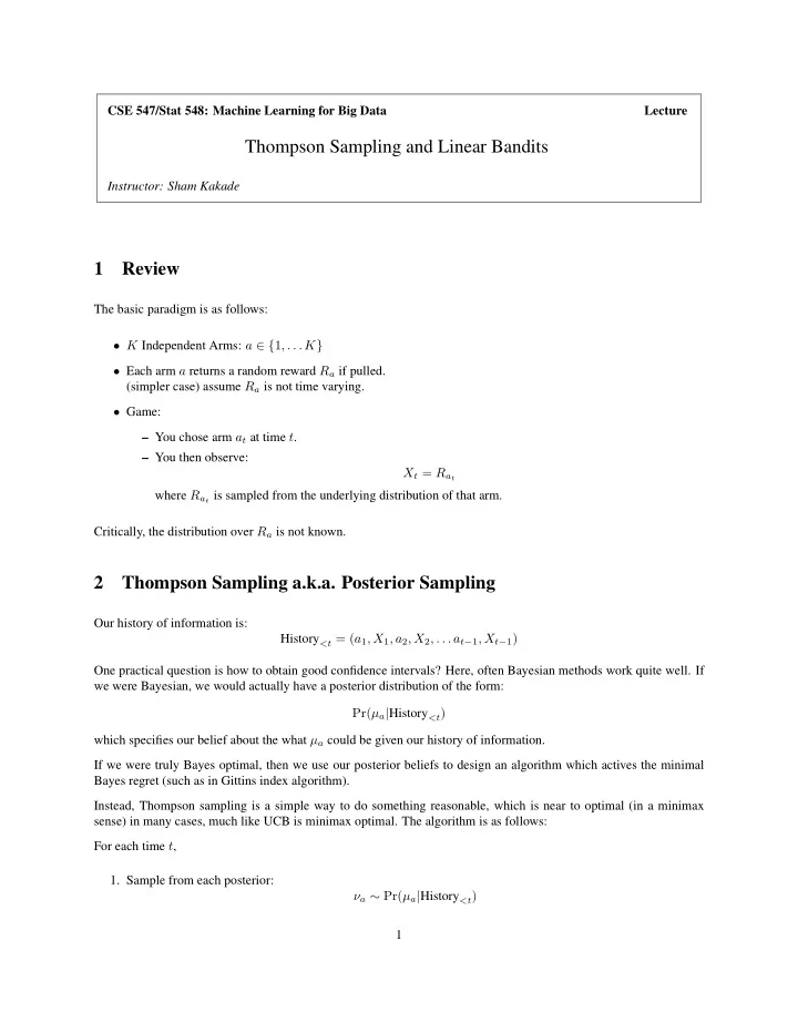
CSE 547/Stat 548: Machine Learning for Big Data Lecture Thompson Sampling and Linear Bandits Instructor: Sham Kakade 1 Review The basic paradigm is as follows: • K Independent Arms: a ∈ { 1 , . . . K } • Each arm a returns a random reward R a if pulled. (simpler case) assume R a is not time varying. • Game: – You chose arm a t at time t . – You then observe: X t = R a t where R a t is sampled from the underlying distribution of that arm. Critically, the distribution over R a is not known. 2 Thompson Sampling a.k.a. Posterior Sampling Our history of information is: History <t = ( a 1 , X 1 , a 2 , X 2 , . . . a t − 1 , X t − 1 ) One practical question is how to obtain good confidence intervals? Here, often Bayesian methods work quite well. If we were Bayesian, we would actually have a posterior distribution of the form: Pr( µ a | History <t ) which specifies our belief about the what µ a could be given our history of information. If we were truly Bayes optimal, then we use our posterior beliefs to design an algorithm which actives the minimal Bayes regret (such as in Gittins index algorithm). Instead, Thompson sampling is a simple way to do something reasonable, which is near to optimal (in a minimax sense) in many cases, much like UCB is minimax optimal. The algorithm is as follows: For each time t , 1. Sample from each posterior: ν a ∼ Pr( µ a | History <t ) 1

2. take action a t = arg max ν a a 3. update our posteriors and go back to 1 . Regret of the Posterior Sampling: In a multi-armed bandit setting (just like for UCB) and under some restriction on our prior, the total expected regret of Thompson sampling is identical to that of the UCB: � T � � � µ ∗ T − E X t ≤ c KT log T t =1 for an appropriately chosen universal constant c . See the related readings for this discussion. 3 Linear Bandits In practice, our space of actions might be very large. The most common way to address this is attempt to embed this space so that there is a linear structure in the reward function. 3.1 The Setting One can view the linear bandits model as an additive effects model (a regression model), where at each round we take a decision x ∈ D ⊂ R d and our payout is linear in this decision. Examples include: • x is path on a graph. • x is a feature vector of properties of an ad • x is which drugs are being prescribed. Upon taking action x , we observe reward r , with expectation: E [ r | x ] = µ ⊤ x Here, we only have d unknown parameters (and “effectively” 2 d actions). As before, we desire an algorithm A (mapping histories to decisions), which has low regret. T � Tµ ⊤ x ∗ − E [ µ ⊤ x t |A ] ≤ ? t =1 (where x ∗ is the best decision) 3.2 The Algorithm: LinUCB We have observed some r 1 , . . . r t − 1 , and have taken Again, let’s think of optimism in the face of uncertainty! x 1 , . . . x t − 1 . Questions: 2

• what is an estimate of the reward of E [ r | x ] and what is our uncertainty? • what is an estimate of µ and what is our uncertainty? We can address these issues using our understanding of regression: Define: � � x τ x ⊤ A t := τ + λI, b t := x τ r τ τ<t τ<t Our estimate of µ is: µ t = A − 1 ˆ t b t and a valid confidence of our estimate: µ t � 2 � µ − ˆ A t ≤ O ( d log t ) (which will hold with probability greater than 1 − poly (1 /t ) ). The algorithm: Define: µ t � 2 B t := { ν |� ν − ˆ A t ≤ O d log t } • At each time t , take action: ν ∈ B t ν ⊤ x x t = arg max x ∈D max then update A t , B t , b t , and ˆ µ t . • Equivalently, take action: � µ ⊤ xA − 1 x t = arg max ˆ t x + ( d log t ) t x x ∈D 3.3 Regret Theorem 3.1. The expected regret bound of LinUCB is bounded as: T √ � Tµ ⊤ x ∗ − E [ µ ⊤ x t ] ≤ O ∗ ( d T ) t =1 (this is the best possible, up to log factors). A few points: √ • compare this to O ( KT ) for the k -arm case • This bound is independent of number of actions. • k -arm case is a special case. • One can also do Thompson sampling as variant of LinUCB, which is a reasonable algorithm in practice. 3