there are two goods, one public ( y ) and one private ( x ) there - PowerPoint PPT Presentation

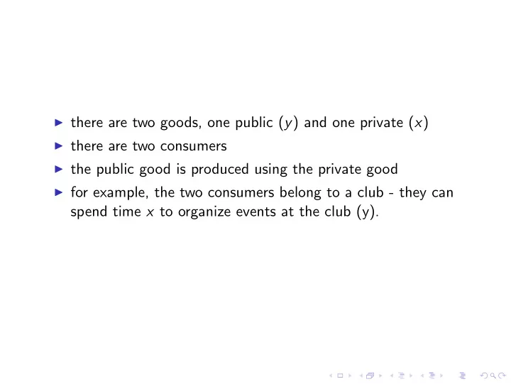
◮ there are two goods, one public ( y ) and one private ( x ) ◮ there are two consumers ◮ the public good is produced using the private good ◮ for example, the two consumers belong to a club - they can spend time x to organize events at the club (y).

◮ the payoffs to the consumers are given by u 1 ( x 1 , y ) for consumer 1 and u 2 ( x 2 , y ) for consumer 2 ◮ x 1 and x 2 are the time that consumer 1 and 2 respectively get to themselves, while y is the total number of events organized by the club - both consumers enjoy all the events at the club equally

◮ events are produced when the two consumers spend time organizing them ◮ the relationship between the number of events and the time each consumer has to themselves is y = f ( ω 1 + ω 2 − x 1 − x 2 ) where ω 1 and ω 2 are the total amount of time that each consumer has to allocate between the two activities ◮ there are no rules about volunteering time, each consumer spends whatever time they like organizing

◮ this is called the voluntary contribution game ◮ the Nash equilibrium is given by a pair of private consumptions x ∗ 1 and x ∗ 2 such that ω 1 + ω 2 − x ′ − x ∗ u 1 ( x ∗ 1 , f ( ω 1 + ω 2 − x ∗ 1 − x ∗ � x ′ , f � �� 2 )) ≥ u 1 2 (1) for any alternative contribution x ′ ∈ [0 , ω 1 ] and u 2 ( x ∗ 2 , f ( ω 1 + ω 2 − x ∗ 1 − x ∗ � x ′ , f � ω 1 + ω 2 − x ∗ 1 − x ′ �� 2 )) ≥ u 2 (2) for any alternative contribution x ′ ∈ [0 , ω 2 ].

◮ in a Nash equilibrium, each consumer believes that he knows how much time the other consumer is going to volunteer ◮ if consumer 1 believes that consumer 2 is going to take x 2 hours for himself, then his or her problem is to maximize u 1 ( x 1 , y ) subject to y = f ( ω 1 + ω 2 − x 1 − x 2 ) . ◮ this is a problem you have seen many many times before - so we can draw a picture

y y = f ( ω 1 + ω 2 ) x ω 1 + ω 2

y y = f ( ω 1 + ω 2 ) x ω 1 + ω 2 x ∗ 2

y y = f ( ω 1 + ω 2 ) f ( ω 1 + ω 2 − x ∗ 2 f ( ω 2 − x ∗ 2 ) x ω 1 ω 1 + ω 2 x ∗ 2

y y = f ( ω 1 + ω 2 ) f ( ω 1 + ω 2 − x ∗ 2 ) ( p, 1) x ω 1 ω 1 + ω 2 x ∗ x ∗ 2 1

y y = f ( ω 1 + ω 2 ) ( p, 1) ( p, 1) x ω 1 ω 1 + ω 2 x ∗ x ∗ 2 1

y y = f ( ω 1 + ω 2 ) f ( ω 1 + ω 2 − x ∗ 2 ) ( p, 1) ( p, 1) ( p, 1) x ω 1 ω 1 + ω 2 x ∗ x ∗ 2 1

Find Equilibrium ◮ in algebra, let u 1 ( x , y ) = α ln ( x ) + (1 − α ) ln ( y ) for both players, and suppose that the production function is just y = ( ω 1 + ω 2 − x 1 − x 2 ). ◮ given his expectation that consumer 2 will contribute ω 2 − x 2 to producing the public good, consumer 1 should solve max x 1 α ln ( x 1 ) + (1 − α ) ln ( ω 1 + ω 2 − x 1 − x 2 ) ◮ the first order condition is (1 − α ) α = ω 1 + ω 2 − x 1 − x 2 x 1 ◮ this gives the simple solution x 1 = α ( ω 1 + ω 2 − x 2 ) .

◮ if you write down the same equation for consumer 2 and solve both equations simultaneously for x 1 and x 2 , you will find they are both the same and equal to 1+ α ( ω 1 + ω 2 ) α ◮ the question we want to ask is - if we (as dictators) could choose x 1 and x 2 to be anything at all, would we be happy with the players choices in a Nash equilibrium? or would we want to try to force them to do something else. ◮ the algebra doesn’t address this question, so lets go back to the diagrams

◮ the equation x 1 = α ( ω 1 + ω 2 − x 2 ) . is player 1’s best reply function ◮ we could draw this on a graph

x 1 R 1 x 2 R 1

x 1 α ( ω 1 + ω 2 ) x 2 ω 1 + ω 2

◮ back to the “what if we could pick anything” approach, we could ask what 1 would do if he could pick both x 1 and x 2 ◮ the he would solve the problem max x 1 , x 2 u 1 ( x 1 , f ( ω 1 + ω 2 − x 1 − x 2 )) ◮ of course that would make him a lot better off ◮ one way to think of the Nash equilibrium is that he does exactly this, but he is constrained to choose x 2 so that it is equal to what he expects 2 to choose

x 1 α ( ω 1 + ω 2 ) R 1 [ x ′′ ] x 2 ω 1 + ω 2 x ′′

x 1 R 1 R 2 x ∗ 1 E x 2 x ∗ R 1 R 2 2

Patents ◮ give player 2 a patent ◮ she controls the public good and charges player 1 for all the public good that is produced ◮ no competition is allowed ◮ if p is the (relative) price of x , the 1 p is the relative price of the public good

y y = f ( ω 1 + ω 2 ) ( p, 1) y ∗ x ω 1 ω 1 + ω 2

y y = f ( ω 1 + ω 2 ) ( p, 1) y ∗ x ω 1 ω 1 + ω 2

y y = f ( ω 1 + ω 2 ) ( p, 1) y ∗ x ω 1 ω 1 + ω 2

y y = f ( ω 1 + ω 2 ) ( p, 1) y ∗ x ω 1 ω 1 + ω 2

y y = f ( ω 1 + ω 2 ) ( p, 1) y ∗ x ω 1 ω 1 + ω 2

y y = f ( ω 1 + ω 2 ) ( p, 1) y ∗ x ω 1 ω 1 + ω 2

y y = f ( ω 1 + ω 2 ) Offer Curve ( p, 1) y ∗ x ω 1 ω 1 + ω 2

y y = f ( ω 1 + ω 2 ) Offer Curve ( p, 1) y ∗ x ω 1 ω 1 + ω 2

y y = f ( ω 1 + ω 2 ) Offer Curve ( p, 1) y ∗ x ω 1 ω 1 + ω 2