Theory of Computation Course note based on Computability, Complexity, - PowerPoint PPT Presentation
Preliminaries (1) Programs and Computable Functions (2) Primitive Recursive Functions (3) A Universal Program (4) Theory of Computation Course note based on Computability, Complexity, and Languages: Fundamentals of Theoretical Computer Science ,
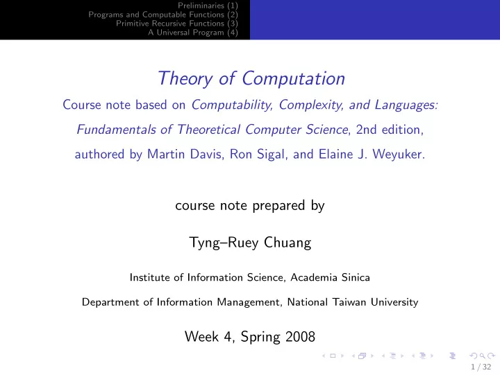
Preliminaries (1) Programs and Computable Functions (2) Primitive Recursive Functions (3) A Universal Program (4) Theory of Computation Course note based on Computability, Complexity, and Languages: Fundamentals of Theoretical Computer Science , 2nd edition, authored by Martin Davis, Ron Sigal, and Elaine J. Weyuker. course note prepared by Tyng–Ruey Chuang Institute of Information Science, Academia Sinica Department of Information Management, National Taiwan University Week 4, Spring 2008 1 / 32
Preliminaries (1) Programs and Computable Functions (2) Primitive Recursive Functions (3) A Universal Program (4) About This Course Note ◮ It is prepared for the course Theory of Computation taught at the National Taiwan University in Spring 2008. ◮ It follows very closely the book Computability, Complexity, and Languages: Fundamentals of Theoretical Computer Science , 2nd edition, by Martin Davis, Ron Sigal, and Elaine J. Weyuker. Morgan Kaufmann Publishers. ISBN: 0-12-206382-1. ◮ It is available from Tyng-Ruey Chuang’s web site: http://www.iis.sinica.edu.tw/~trc/ and released under a Creative Commons “Attribution-ShareAlike 2.5 Taiwan” license: http://creativecommons.org/licenses/by-sa/2.5/tw/ 2 / 32
Preliminaries (1) Programs and Computable Functions (2) Functions (1.2) Primitive Recursive Functions (3) A Universal Program (4) One-One Functions ◮ A function is one-one if, for all x , y in the domain of f , f ( x ) = f ( y ) implies x = y . ◮ That is, if x � = y , then f ( x ) � = f ( y ). ◮ Function f ( n ) = n 2 is one-one. ◮ Function u 2 1 ( x 1 , x 2 ) = x 1 is not one-one as, for example, both u 2 1 (0 , 0) and u 2 1 (0 , 1) map to 0. 3 / 32
Preliminaries (1) Programs and Computable Functions (2) Functions (1.2) Primitive Recursive Functions (3) A Universal Program (4) Onto Functions ◮ If the range of f is the set S , then we say f is an onto function with respect to S , or simply that f is onto S . ◮ Function f ( n ) = n 2 is onto the set of perfect squares { n 2 | n ∈ N } , but is not onto N . ◮ Let S 1 × S 2 be domain of function u 2 1 ( x 1 , x 2 ) = x 1 , then function u 2 1 ( x 1 , x 2 ) is onto S 1 . 4 / 32
Preliminaries (1) Programs and Computable Functions (2) Computable Functions (2.4) Primitive Recursive Functions (3) A Universal Program (4) Programs Accepting Any Number of Inputs ◮ We permit each program to be used with any number of inputs. ◮ If the program has n input variables, but only m < n are specified, the remaining n − m input variables are assigned the value 0 and the computation proceeds. ◮ On the other hand, if m > n values are specified, then the extra input values are ignored. 5 / 32
Preliminaries (1) Programs and Computable Functions (2) Computable Functions (2.4) Primitive Recursive Functions (3) A Universal Program (4) Programs Accepting Any Number of Inputs, Examples ◮ Consider the following program P that computes x 1 + x 2 , Y ← X 1 Z ← X 2 [ B ] IF Z � = 0 GOTO A GOTO E [ A ] Z ← Z − 1 Y ← Y + 1 GOTO B ◮ We have Ψ (1) P ( r 1 ) = r 1 + 0 = r 1 Ψ (3) P ( r 1 , r 2 , r 3 ) = r 1 + r 2 6 / 32
Preliminaries (1) Programs and Computable Functions (2) Pairing Functions and G¨ odel Numbers (3.9) Primitive Recursive Functions (3) A Universal Program (4) Pairing Functions ◮ There is a one-one and onto function from N × N to N (with domain N × N and range N ). This function is called a pairing function. ◮ That is, we can map a pair of numbers to a single number, and back, without losing information. Likewise, we can compute from any number a pair of numbers, and back, without missing anything. ◮ The primitive recursive function � x , y � = 2 x (2 y + 1) ˙ − 1 is a pairing function. ◮ � 0 , 0 � = 0 , � 1 , 0 � = 1 , � 0 , 1 � = 2 , . . . 7 / 32
Preliminaries (1) Programs and Computable Functions (2) Pairing Functions and G¨ odel Numbers (3.9) Primitive Recursive Functions (3) A Universal Program (4) The Pairing Function � x , y � = 2 x (2 y + 1) ˙ − 1 ◮ Note that 2 x (2 y + 1) � = 0, so � x , y � + 1 = 2 x (2 y + 1) ◮ If z is any given number, then there is a unique solution x , y to the equation � x , y � = z . ◮ Namely, x is the largest number such that 2 x | ( z + 1), and y is then the solution of the equation 2 y + 1 = ( z + 1) / 2 x . ◮ The pairing function thus defines two functions l and r such that x = l ( z ) and y = r ( z ). 8 / 32
Preliminaries (1) Programs and Computable Functions (2) Pairing Functions and G¨ odel Numbers (3.9) Primitive Recursive Functions (3) A Universal Program (4) The Pairing Function � x , y � = 2 x (2 y + 1) ˙ − 1, Continued If � x , y � = z , then x , y < z + 1. Hence, l ( z ) ≤ z , and r ( z ) ≤ z . We can write l ( z ) = min x ≤ z [( ∃ y ) ≤ z ( z = � x , y � )] , r ( z ) = min y ≤ z [( ∃ x ) ≤ z ( z = � x , y � )] , so that l ( z ) and r ( z ) are primitive recursive functions. 9 / 32
Preliminaries (1) Programs and Computable Functions (2) Pairing Functions and G¨ odel Numbers (3.9) Primitive Recursive Functions (3) A Universal Program (4) Pairing Function Theorem Theorem 8.1. The functions � x , y � , l ( z ) , and r ( z ) have the following properties: 1. they are primitive recursive; 2. l ( � x , y � ) = x , r ( � x , y � ) = y ; 3. � l ( z ) , r ( z ) � = z ; 4. l ( z ) , r ( z ) ≤ z . 10 / 32
Preliminaries (1) Programs and Computable Functions (2) Pairing Functions and G¨ odel Numbers (3.9) Primitive Recursive Functions (3) A Universal Program (4) G¨ odel Number We define the G¨ odel Number of the sequence ( a 1 , . . . , a n ) to be the number n � p a i [ a 1 , . . . , a n ] = i i =1 Thus, the the G¨ odel number of the sequence (3, 1, 5, 4, 6) is [3 , 1 , 5 , 4 , 6] = 2 3 · 3 1 · 5 5 · 7 4 · 11 6 For each fixed n , the function [ a 1 , . . . , a n ] is clearly primitive recursive. Note that the G¨ odel numbering method encodes and decodes arbitrary finite sequences of numbers. 11 / 32
Preliminaries (1) Programs and Computable Functions (2) Pairing Functions and G¨ odel Numbers (3.9) Primitive Recursive Functions (3) A Universal Program (4) Uniqueness Property of G¨ odel Numbering Theorem 8.2. If [ a 1 , . . . , a n ] = [ b 1 , . . . , b n ], then a i = b i for all i = 1 , . . . , n . � This result is an immediate consequence of the uniqueness of the factorization of integers into primes, sometimes referred to as the unique factorization theorem . Note that, 1 = 2 0 = 2 0 3 0 = 2 0 3 0 5 0 = . . . , hence it is natural to regard 1 as the G¨ odel number of the “empty” sequence (i.e., the sequence of length 0). 12 / 32
Preliminaries (1) Programs and Computable Functions (2) Pairing Functions and G¨ odel Numbers (3.9) Primitive Recursive Functions (3) A Universal Program (4) Function ( x ) i We now define a primitive recursive function ( x ) i so that if x = [ a 1 , . . . , a n ] then ( x ) i = a i . We set t ≤ x ( ∼ p t +1 ( x ) i = min | x ) i Note that ( x ) 0 = 0, and (0) i = 0 for all i . 13 / 32
Preliminaries (1) Programs and Computable Functions (2) Pairing Functions and G¨ odel Numbers (3.9) Primitive Recursive Functions (3) A Universal Program (4) Function Lt ( x ) We also define the “length” function Lt , Lt ( x ) = min i ≤ x [( x ) i � = 0 & ( ∀ j ) ≤ x ( j ≤ i ∨ ( x ) j = 0)] For example, if x = 20 = 2 2 · 5 1 = [2 , 0 , 1] then ( x ) 1 = 2 , ( x ) 2 = 0 , ( x ) 3 = 1, but ( x ) 4 = 0 , ( x ) 5 = 0 , . . . , ( x ) i = 0, for all i ≥ 4. So Lt (20) = 3. Note that Lt (0) = Lt (1) = 0. If x > 1, and Lt ( x ) = n , then p n divides x but no prime greater than p n divides x . 14 / 32
Preliminaries (1) Programs and Computable Functions (2) Pairing Functions and G¨ odel Numbers (3.9) Primitive Recursive Functions (3) A Universal Program (4) Sequence Number Theorem Theorem 8.3. 1. � a i if 1 ≤ i ≤ n ([ a 1 , . . . , a n ]) i = 0 otherwise. 2. [( x ) 1 , . . . , ( x ) n ] = x if n ≥ Lt ( x ) . � 15 / 32
Preliminaries (1) Programs and Computable Functions (2) Coding Programs by Numbers (4.1) Primitive Recursive Functions (3) The Halting Problem (4.2) A Universal Program (4) Coding Programs by Numbers For each program P in language S , we will devise a method ◮ to associate a unique number, #( P ), to the program P , and ◮ to retrieve a program from its number. In addition, for each number n ∈ N , we will retrieve from n a program. 16 / 32
Preliminaries (1) Programs and Computable Functions (2) Coding Programs by Numbers (4.1) Primitive Recursive Functions (3) The Halting Problem (4.2) A Universal Program (4) Arranging Variables and Labels ◮ The variables are arranged in the following order Y , X 1 , Z 1 , X 2 , Z 2 , X 3 , Z 3 , . . . ◮ The labels are arranged in the following order A 1 , B 1 , C 1 , D 1 , E 1 , A 2 , B 2 , C 2 , D 2 , E 2 , A 3 , . . . ◮ #( V ) is the position of variable V in the ordering. So is #( L ) for label L . ◮ Thus, #( X 2 ) = 4 , #( Z 1 ) = #( Z ) = 3 , #( E ) = 5 , #( B 2 ) = 7 , . . . . 17 / 32
Recommend
More recommend
Explore More Topics
Stay informed with curated content and fresh updates.
