randomized computation Sometimes randomness helps in computation. - PowerPoint PPT Presentation

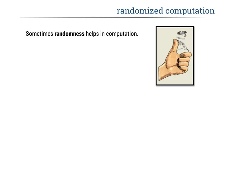
randomized computation Sometimes randomness helps in computation.

randomized computation Augment our usual Turing machines with a read-only tape of random bits . 𝑟 start 𝑟 0 𝑟 2 𝑟 accept 𝑟 1 # # 𝑐 𝑏 𝑏 𝑏 0 1 1 0 0 0 1 1

randomized computation The notion of acceptance changes. What does it mean for a TM 𝑁 with access to random bits to decide a language 𝑀 ? One-sided error [two variants]: 1 𝑦 ∈ 𝑀 ⇒ Pr 𝑁 accepts 𝑦 = 1 𝑦 ∈ 𝑀 ⇒ Pr 𝑁 accepts 𝑦 > 10 9 𝑦 ∉ 𝑀 ⇒ Pr 𝑁 accepts 𝑦 < 𝑦 ∉ 𝑀 ⇒ Pr 𝑁 accepts 𝑦 = 0 10 Two-sided error: 2 In both cases, we can make 𝑦 ∈ 𝑀 ⇒ Pr 𝑁 accepts 𝑦 > 3 the error much smaller by 1 𝑦 ∉ 𝑀 ⇒ Pr 𝑁 accepts 𝑦 < repeating a few times. 3

randomized computation For instance, the two-sided error variant of 𝐐 is called 𝐂𝐐𝐐 . 𝐂𝐐𝐐 stands for “bounded - error probabilistic polynomial time” Derandomization problem: Can every efficient randomized algorithm be replaced by a deterministic one? We don’t know the answer, though it is expected to be “yes.” This is the question of 𝐐 vs. 𝐂𝐐𝐐 .

randomized computation Recall the complexity class 𝐌 = SPACE log 𝑜 The randomized one-sided error variant of 𝐌 is called 𝐒𝐌 . A language 𝐵 is in 𝐒𝐌 if there is a randomized 𝑃 log 𝑜 space Turing machine such that [one way access to random tape]: 1 𝑦 ∈ 𝐵 ⇒ Pr 𝑁 accepts 𝑦 ≥ 2 𝑦 ∉ 𝐵 ⇒ Pr 𝑁 accepts 𝑦 = 0 The question of whether 𝐌 = 𝐒𝐌 is also open . We know that 𝐒𝐌 ⊆ 𝐎𝐌 ⊆ SPACE log 𝑜 2 Nisan showed how to do this using a pseudo-random number generator for space-bounded machines.

undirected connectivity Recall the language: DIRPATH = 𝐻, 𝑡, 𝑢 ∶ 𝐻 is a directed graph with a directed 𝑡 → 𝑢 path We saw that DIRPATH is 𝐎𝐌 -complete. Thus 𝐌 = 𝐎𝐌 if and only if DIRPATH ∈ 𝑴 . What about the language? PATH = 𝐻, 𝑡, 𝑢 ∶ 𝐻 is an 𝐯𝐨𝐞𝐣𝐬𝐟𝐝𝐮𝐟𝐞 graph with an 𝑡 ↔ 𝑢 path

undirected connectivity What about the language? PATH = 𝐻, 𝑡, 𝑢 ∶ 𝐻 is an 𝐯𝐨𝐞𝐣𝐬𝐟𝐝𝐮𝐟𝐞 graph with an 𝑡 ↔ 𝑢 path Is PATH ∈ 𝐌 ?

random walks Let’s show that PATH ∈ 𝐒𝐌 . One step of random walk : Move to a uniformly random neighbor.

random walks What we will show: If 𝐻 = (𝑊, 𝐹) is a graph with 𝑜 vertices and 𝑛 edges, then a random walker started at 𝑡 ∈ 𝑊 who takes 4𝑛𝑜 steps will visit every vertex in the connected component of 𝑡 with probability at least ½ . In particular, if there is an 𝑡 ↔ 𝑢 path in 𝐻 , she will visit 𝑢 with probability at least ½ .

random walks What we will show: If 𝐻 = (𝑊, 𝐹) is a graph with 𝑜 vertices and 𝑛 edges, then a random walker started at 𝑡 ∈ 𝑊 who takes 4𝑛𝑜 steps will visit every vertex in the connected component of 𝑡 with probability at least ½ . In particular, if there is an 𝑡 ↔ 𝑢 path in 𝐻 , she will visit 𝑢 with probability at least ½ . 𝐒𝐌 Algorithm: Start a random walker at 𝑡 and use the random bits to simulate a random walk for 4𝑛𝑜 steps (can count this high in 𝑃 log 𝑜 space). If we visit 𝑢 at any point, accept. Otherwise, reject. 1 If there is an 𝑡 ↔ 𝑢 path in 𝐻 : Pr accept 𝐻, 𝑡, 𝑢 ≥ 2 If no 𝑡 ↔ 𝑢 path in 𝐻 : Pr accept 𝐻, 𝑡, 𝑢 = 0

cover time of a graph Cover time of a graph = expected # of steps before all vertices are visited.

cover time of a graph We will show that if 𝐻 has 𝑜 vertices and 𝑛 then the expected time before the random walk covers 𝐻 (from any starting point) is 2𝑛𝑜. Then it must be that with probability at least ½ , we cover 𝐻 after 4𝑛𝑜 steps. (This fact is called “Markov’s inequality.”)

heat dispersion on a graph

spectral embedding 𝑤 2

hitting times and commute times For vertices 𝑣, 𝑤 ∈ 𝑊 , the hitting time is 𝐼 𝑣, 𝑤 = expected time for random walk to hit 𝑤 starting at 𝑣 The commute time between 𝑣 and 𝑤 is 𝐷 𝑣, 𝑤 = 𝐼 𝑣, 𝑤 + 𝐼(𝑤, 𝑣) 𝑣 𝑤

hitting times and commute times For vertices 𝑣, 𝑤 ∈ 𝑊 , the hitting time is 𝐼 𝑣, 𝑤 = expected time for random walk to hit 𝑤 starting at 𝑣 The commute time between 𝑣 and 𝑤 is 𝐷 𝑣, 𝑤 = 𝐼 𝑣, 𝑤 + 𝐼(𝑤, 𝑣) Claim: If {𝑣, 𝑤} is an edge of 𝐻 , then 𝐷 𝑣, 𝑤 ≤ 2𝑛 . 𝑣 𝑤

hitting times and commute times Claim: If {𝑣, 𝑤} is an edge of 𝐻 , then 𝐷 𝑣, 𝑤 ≤ 2𝑛 . Let’s use the claim to show that the cover time of 𝐻 is at most 2𝑛(𝑜 − 1) . 𝑡

hitting times and commute times Claim: If {𝑣, 𝑤} is an edge of 𝐻 , then 𝐷 𝑣, 𝑤 ≤ 2𝑛 . Let’s use the claim to show that the cover time of 𝐻 is at most 2𝑛(𝑜 − 1) . 𝑡 Choose an arbitrary spanning tree of 𝐻 .

hitting times and commute times Claim: If {𝑣, 𝑤} is an edge of 𝐻 , then 𝐷 𝑣, 𝑤 ≤ 2𝑛 . Let’s use the claim to show that the cover time of 𝐻 is at most 2𝑛(𝑜 − 1) . 𝑡 Choose an arbitrary spanning tree of 𝐻 . Consider the “tour around the spanning tree” This is a path 𝑡 = 𝑣 0 , 𝑣 1 , 𝑣 2 , … , 𝑣 2𝑜 = 𝑡 Where 𝑣 𝑗 , 𝑣 𝑗+1 is an edge for each 𝑗 , and each edge appears exactly twice.

hitting times and commute times Claim: If {𝑣, 𝑤} is an edge of 𝐻 , then 𝐷 𝑣, 𝑤 ≤ 2𝑛 . Let’s use the claim to show that the cover time of 𝐻 is at most 2𝑛(𝑜 − 1) . 𝑡 Choose an arbitrary spanning tree of 𝐻 . Consider the “tour around the spanning tree” Claim: Cover time of 𝐻 is at most 𝐷 𝑣 0 , 𝑣 1 + 𝐷 𝑣 1 , 𝑣 2 + 𝐷 𝑣 2 , 𝑣 3 + ⋯ + 𝐷 𝑣 2𝑜−1 , 𝑣 2𝑜

hitting times and commute times Claim: If {𝑣, 𝑤} is an edge of 𝐻 , then 𝐷 𝑣, 𝑤 ≤ 2𝑛 . Let’s use the claim to show that the cover time of 𝐻 is at most 2𝑛(𝑜 − 1) . 𝑡 Choose an arbitrary spanning tree of 𝐻 . Consider the “tour around the spanning tree” Claim: Cover time of 𝐻 is at most 𝐷(𝑣, 𝑤) ≤ 2𝑛(𝑜 − 1) 𝑣,𝑤 ∈𝑈

high school physics Claim: If {𝑣, 𝑤} is an edge of 𝐻 , then 𝐷 𝑣, 𝑤 ≤ 2𝑛 .

high school physics Claim: If {𝑣, 𝑤} is an edge of 𝐻 , then 𝐷 𝑣, 𝑤 ≤ 2𝑛 . View the graph 𝐻 as an electrical network with unit resistances on the edges. When a potential difference is applied between the nodes from an external source, current flows in the network in accordance with Kirchoff’s and Ohm’s laws. K1: The total current flowing into a vertex = total current flowing out K2: The sum of potential differences around any cycle is zero. Ohm: The current flowing along any edge {𝑣, 𝑤} is equal to (potential 𝑣 − potential 𝑤 )/resistance(𝑣, 𝑤) 𝑣 The effective resistance between 𝑣 and 𝑤 is 𝑤 defined as the potential difference required to send one unit of current from 𝑣 to 𝑤 .

presentation agenda Simple uses of randomness in computation: 1. Checking matrix multiplication [Mahmoud] 2. Karp-Rabin matching algorithm [Stanislav] random Error-correcting codes: 1. Intro [Amr] 2. Reed-Solmon codes [Jie] 3. Expander codes [Ali] pseudo-random