Model of Computation and Runtime Analysis Model of Computation - PowerPoint PPT Presentation
Model of Computation and Runtime Analysis Model of Computation Model of Computation Specifies Set of operations Cost of operations (not necessarily time) Examples Turing Machine Random Access Machine (RAM) PRAM Map
Model of Computation and Runtime Analysis
Model of Computation
Model of Computation Specifies ◮ Set of operations ◮ Cost of operations (not necessarily time) Examples ◮ Turing Machine ◮ Random Access Machine (RAM) ◮ PRAM ◮ Map Reduce(?) 3 / 18
Random Access Machine Word ◮ Group of constant number of bits (e. g. byte) ◮ ≥ log ( input size ) ◮ Usually integers or floats Memory ◮ Big array of words ◮ Access by address Operations ◮ Read and write a word from or into memory ◮ Arithmetic + , − , ∗ , / , mod , ⌊ ⌋ ◮ Logic (can be bitwise) ∧ , ∨ , xor , ¬ ◮ Comparison based decisions Each operation cost 1 unit of time. 4 / 18
Asymptotic Complexity
Asymptotic Complexity Goal ◮ Determine runtime of an algorithm. Depends on ◮ Input ◮ Hardware ◮ Programming language, compiler, and runtime environment Solution ◮ Asymptotic Complexity ◮ How does the runtime behave based on the input size n ? 6 / 18
Asymptotic Complexity Hardware ◮ Raspberry Pi 2B 0.9 GHz ◮ Nexus 5 2.3 GHz ◮ Intel i7 4.0 GHz ◮ Same for other components (e.g. memory) Runtime Environment ◮ Machine code (e. g. C++) ◮ Managed code (e. g. C#/Java) ◮ Interpreted code (e. g. Python) ◮ Virtual Machines (e. g. VirtualBox) Conclusion ◮ Ignore constant factors. 7 / 18
Asymptotic Complexity Consider two algorithms ◮ T 1 ( n ) = n 2 + 5 n + 5 ◮ T 2 ( n ) = n 2 n 4 16 64 256 1024 4096 T 1 ( n ) 41 341 4 , 421 66 , 821 1 , 053 , 701 16 , 797 , 701 T 2 ( n ) 16 256 4 , 096 65 , 536 1 , 048 , 576 16 , 777 , 216 T 1 / T 2 2 . 5625 1 . 332 1 . 0793 1 . 0196 1 . 0049 1 . 0012 Conclusion ◮ Only keep strongest part. ( n 2 in this case) 8 / 18
Example Consider two algorithms and two computers ◮ Fast computer and slow algorithm 10 7 operations per second T 1 ( n ) = n 2 ◮ Slow computer and fast algorithm 10 4 operations per second T 2 ( n ) = n ⌈ log 2 n ⌉ ◮ Input size: 10 6 Runtime ◮ T 1 = ( 10 6 ) 2 s = 10 5 s ≈ 27 . 8 h 10 7 ◮ T 2 = 10 6 ⌈ log 2 10 6 ⌉ s = 2 , 000 s ≈ 33 . 3 min 10 4 Conclusion ◮ First lower complexity, then constant factors. 9 / 18
Big-O Notation Based on complexity, 3 n 2 − log 2 n , and n 2 + 5 n + 5 are the same as n 2 . How do we write this? Big-O Notation ◮ O ( g ) = { f : N → N | ∃ c > 0 ∃ n 0 > 0 ∀ n ≥ n 0 : f ( n ) ≤ c · g ( n ) } ◮ f ∈ O ( g ) means g is an upper bound for f . ◮ O ( 3 n 2 − log n ) = O ( n 2 + 5 n + 5 ) = O ( n 2 ) If an algorithm has runtime n 2 + 5 n + 5 , we say it runs in O ( n 2 ) time. Note that O ( n ) ⊂ O ( n log n ) ⊂ O ( n 2 ) 10 / 18
Common Examples Complexity Example O ( 1 ) constant basic operations O ( log n ) logarithmic binary search O ( n ) linear counting, linear search, DFS/BFS O ( n log n ) sorting, finding doubles, convex hull O ( n 2 ) quadratic checking all pairs � 2 log c n � Graph Isomorphism † O quasi polynomial O ( 2 n ) exponential SAT O ( n !) checking all permutations † Preliminary result, not peer reviewed yet. 11 / 18
Big-O Notation — f ∈ O ( g ) f ∈ O ( g ) : g is an upper bound for f . ◮ ∃ c > 0 ∃ n 0 > 0 ∀ n ≥ n 0 : f ( n ) ≤ c · g ( n ) c · g f n 0 12 / 18
Big-O Notation — f ∈ Ω( g ) f ∈ Ω( g ) : g is a lower bound for f . ◮ ∃ c > 0 ∃ n 0 > 0 ∀ n ≥ n 0 : f ( n ) ≥ c · g ( n ) ◮ f ∈ Ω( g ) ↔ g ∈ O ( f ) f c · g n 0 13 / 18
Big-O Notation — f ∈ Θ( g ) f ∈ Θ( g ) ◮ ∃ c 1 , c 2 > 0 ∃ n 0 > 0 ∀ n ≥ n 0 : c 1 · g ( n ) ≤ f ( n ) ≤ c 2 · g ( n ) ◮ Θ( g ) = O ( g ) ∩ Ω( g ) c 2 · g f c 1 · g n 0 14 / 18
Big-O Notation — f ∈ o ( g ) f ∈ o ( g ) : f is dominated by g . ◮ ∀ c > 0 ∃ n 0 > 0 ∀ n ≥ n 0 : f ( n ) ≤ c · g ( n ) (This includes c ≤ 1 .) g f n 0 15 / 18
Big-O Notation f ∈ O ( g ) : g is an upper bound for f . ◮ ∃ c > 0 ∃ n 0 > 0 ∀ n ≥ n 0 : f ( n ) ≤ c · g ( n ) f ∈ Ω( g ) : g is a lower bound for f . ◮ ∃ c > 0 ∃ n 0 > 0 ∀ n ≥ n 0 : f ( n ) ≥ c · g ( n ) ◮ f ∈ Ω( g ) ↔ g ∈ O ( f ) f ∈ Θ( g ) ◮ ∃ c 1 , c 2 > 0 ∃ n 0 > 0 ∀ n ≥ n 0 : c 1 · g ( n ) ≤ f ( n ) ≤ c 2 · g ( n ) ◮ Θ( g ) = O ( g ) ∩ Ω( g ) f ∈ o ( g ) : f is dominated by g . ◮ ∀ c > 0 ∃ n 0 > 0 ∀ n ≥ n 0 : f ( n ) ≤ c · g ( n ) (This includes c ≤ 1 .) 16 / 18
Questions True or False? Explain your answer. a) f ∈ O ( g ) implies g ∈ O ( f ) b) f + g ∈ Θ( min ( f , g )) c) f ∈ O ( g ) implies log f ∈ O ( log g ) d) f ∈ O ( g ) implies 2 f ∈ O ( 2 g ) e) f ∈ O ( f 2 ) f) f ∈ O ( g ) implies g ∈ Ω( f ) g) f ( n ) ∈ Θ( f ( n / 2 )) h) g ∈ o ( f ) implies f + g ∈ Θ( f ) 17 / 18
Questions Rank the following functions by order of growth. Partition your list into equivalence classes such that functions f i and f j are in the same class if and only if f i ∈ Θ( f j ) . � √ � 3 � log n � n log 2 n n 2 2 n ! 2 2 2 n n 1 / log n n · 2 n log log n log n n log log n n 3 2 log n ( log n ) log n 1 2 2 n + 1 4 log n 2 n n n log n 18 / 18
Recommend
More recommend
Explore More Topics
Stay informed with curated content and fresh updates.

