Theorem: If a range space S = ( P, R ) over a set P of size n has - PDF document

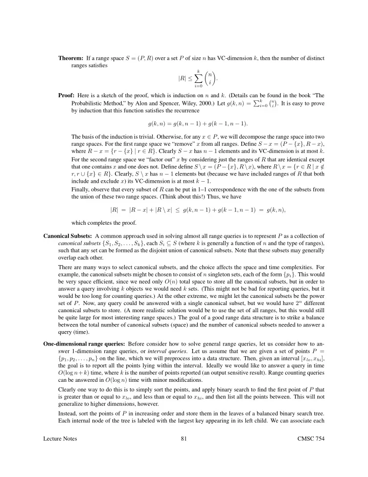
Theorem: If a range space S = ( P, R ) over a set P of size n has VC-dimension k , then the number of distinct ranges satisfies k � n � � | R | ≤ . i i =0 Proof: Here is a sketch of the proof, which is induction on n and k . (Details can be found in the book “The Probabilistic Method,” by Alon and Spencer, Wiley, 2000.) Let g ( k, n ) = � k � n � . It is easy to prove i =0 i by induction that this function satisfies the recurrence g ( k, n ) = g ( k, n − 1) + g ( k − 1 , n − 1) . The basis of the induction is trivial. Otherwise, for any x ∈ P , we will decompose the range space into two range spaces. For the first range space we “remove” x from all ranges. Define S − x = ( P − { x } , R − x ) , where R − x = { r − { x } | r ∈ R } . Clearly S − x has n − 1 elements and its VC-dimension is at most k . For the second range space we “factor out” x by considering just the ranges of R that are identical except that one contains x and one does not. Define define S \ x = ( P −{ x } , R \ x ) , where R \ x = { r ∈ R | x / ∈ r, r ∪ { x } ∈ R } . Clearly, S \ x has n − 1 elements but (because we have included ranges of R that both include and exclude x ) its VC-dimension is at most k − 1 . Finally, observe that every subset of R can be put in 1–1 correspondence with the one of the subsets from the union of these two range spaces. (Think about this!) Thus, we have | R | = | R − x | + | R \ x | ≤ g ( k, n − 1) + g ( k − 1 , n − 1) = g ( k, n ) , which completes the proof. Canonical Subsets: A common approach used in solving almost all range queries is to represent P as a collection of canonical subsets { S 1 , S 2 , . . . , S k } , each S i ⊆ S (where k is generally a function of n and the type of ranges), such that any set can be formed as the disjoint union of canonical subsets. Note that these subsets may generally overlap each other. There are many ways to select canonical subsets, and the choice affects the space and time complexities. For example, the canonical subsets might be chosen to consist of n singleton sets, each of the form { p i } . This would be very space efficient, since we need only O ( n ) total space to store all the canonical subsets, but in order to answer a query involving k objects we would need k sets. (This might not be bad for reporting queries, but it would be too long for counting queries.) At the other extreme, we might let the canonical subsets be the power set of P . Now, any query could be answered with a single canonical subset, but we would have 2 n different canonical subsets to store. (A more realistic solution would be to use the set of all ranges, but this would still be quite large for most interesting range spaces.) The goal of a good range data structure is to strike a balance between the total number of canonical subsets (space) and the number of canonical subsets needed to answer a query (time). One-dimensional range queries: Before consider how to solve general range queries, let us consider how to an- swer 1-dimension range queries, or interval queries . Let us assume that we are given a set of points P = { p 1 , p 2 , . . . , p n } on the line, which we will preprocess into a data structure. Then, given an interval [ x lo , x hi ] , the goal is to report all the points lying within the interval. Ideally we would like to answer a query in time O (log n + k ) time, where k is the number of points reported (an output sensitive result). Range counting queries can be answered in O (log n ) time with minor modifications. Clearly one way to do this is to simply sort the points, and apply binary search to find the first point of P that is greater than or equal to x lo , and less than or equal to x hi , and then list all the points between. This will not generalize to higher dimensions, however. Instead, sort the points of P in increasing order and store them in the leaves of a balanced binary search tree. Each internal node of the tree is labeled with the largest key appearing in its left child. We can associate each Lecture Notes 81 CMSC 754

node of this tree (implicitly or explicitly) with the subset of points stored in the leaves that are descendents of this node. This gives rise to the O ( n ) canonical subsets . For now, these canonical subsets will not be stored explicitly as part of the data structure, but this will change later when we talk about range trees. This is illustrated in the figure below. 15 24 7 {9,12,14,15} 3 12 20 27 {4,7} {17,20} 4 9 14 17 22 25 29 1 {3} {22} 1 3 4 7 9 12 14 15 17 20 22 24 25 27 29 31 u v x =2 x =23 lo hi Figure 66: Canonical sets for interval queries. We claim that the canonical subsets corresponding to any range can be identified in O (log n ) time from this structure. Given any interval [ x lo , x hi ] , we search the tree to find the leftmost leaf u whose key is greater than or equal to x lo and the rightmost leaf v whose key is less than or equal to x hi . Clearly all the leaves between u and v , together possibly with u and v , constitute the points that lie within the range. If key ( u ) = x lo then we include u ’s canonical (single point) subset and if key ( v ) = x hi then we do the same for v . To form the remaining canonical subsets, we take the subsets of all the maximal subtrees lying between u and v . Here is how to compute these subtrees. The search paths to u and v may generally share some common subpath, starting at the root of the tree. Once the paths diverge, as we follow the left path to u , whenever the path goes to the left child of some node, we add the canonical subset associated with its right child. Similarly, as we follow the right path to v , whenever the path goes to the right child, we add the canonical subset associated with its left child. To answer a range reporting query we simply traverse these canonical subtrees, reporting the points of their leaves. Each tree can be traversed in time proportional to the number of leaves in each subtree. To answer a range counting query we store the total number of points in each subtree (as part of the preprocessing) and then sum all of these over all the canonical subtrees. Since the search paths are of length O (log n ) , it follows that O (log n ) canonical subsets suffice to represent the answer to any query. Thus range counting queries can be answered in O (log n ) time. For reporting queries, since the leaves of each subtree can be listed in time that is proportional to the number of leaves in the tree (a basic fact about binary trees), it follows that the total time in the search is O (log n + k ) , where k is the number of points reported. In summary, 1-dimensional range queries can be answered in O (log n ) time, using O ( n ) storage. This concept of finding maximal subtrees that are contained within the range is fundamental to all range search data structures. The only question is how to organize the tree and how to locate the desired sets. Let see next how can we extend this to higher dimensional range queries. Kd-trees: The natural question is how to extend 1-dimensional range searching to higher dimensions. First we will consider kd-trees. This data structure is easy to implement and quite practical and useful for many different types of searching problems (nearest neighbor searching for example). However it is not the asymptotically most efficient solution for the orthogonal range searching, as we will see later. Lecture Notes 82 CMSC 754