The Wealth Distribution and the MPC: Implications of the New EU - PowerPoint PPT Presentation
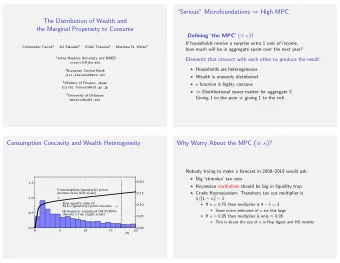
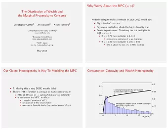
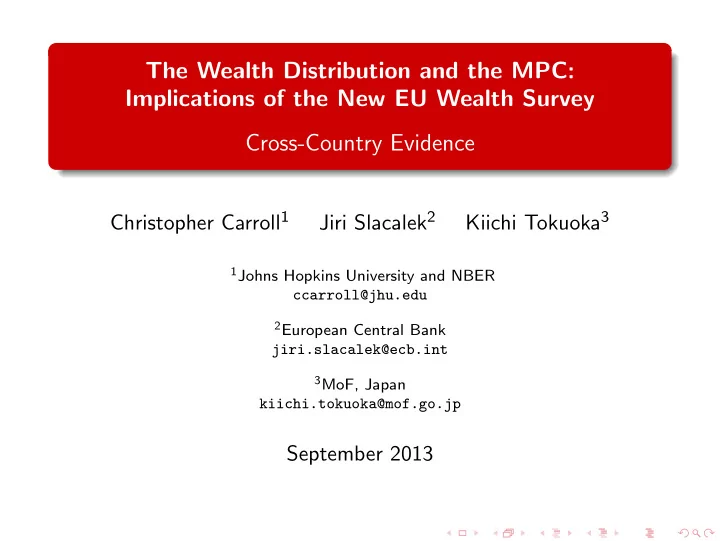
The Wealth Distribution and the MPC: Implications of the New EU Wealth Survey Cross-Country Evidence Christopher Carroll 1 Jiri Slacalek 2 Kiichi Tokuoka 3 1 Johns Hopkins University and NBER ccarroll@jhu.edu 2 European Central Bank
The Wealth Distribution and the MPC: Implications of the New EU Wealth Survey Cross-Country Evidence Christopher Carroll 1 Jiri Slacalek 2 Kiichi Tokuoka 3 1 Johns Hopkins University and NBER ccarroll@jhu.edu 2 European Central Bank jiri.slacalek@ecb.int 3 MoF, Japan kiichi.tokuoka@mof.go.jp September 2013
References Motivation Wealth inequality: substantial and varying across countries (b) Ginis for Net Wealth (a) Lorenz Curves for Income/Net Wealth, US/Euro Area Carroll, Slacalek and Tokuoka The Distribution of Wealth and the MPC:
References How Should Differences in Wealth/Income Relate to the MPC? To-Do List Simulate a standard consumption/saving model (with permanent/transitory income a la Carroll, Slacalek, and Tokuoka (2013)) Match model to each country’s wealth distribution and income dynamics Back out implications for marginal propensity to consume, MPC Carroll, Slacalek and Tokuoka The Distribution of Wealth and the MPC:
References Findings—Heterogeneity Matters! Model Implications 1 Important to match wealth distribution 2 High MPC out of transitory income shocks Particularly high MPC when matching liquid assets High MPC for low-wealth/low-income/unemployed households Wealth inequality increases economy’s MPC ⇒ MPC in US = 0 . 2–0 . 6 > MPC in Europe = 0 . 1–0 . 4 MPC higher under larger transitory income shocks 3 In line with empirical evidence on MPC but in stark contrast w/ repr-agent models (MPC ∼ 0 . 02–0.04) Carroll, Slacalek and Tokuoka The Distribution of Wealth and the MPC:
References Wealth Distribution and Concavity of Consumption Function 0.2 1.5 Consumption �� quarterly � permanent income ratio � left scale � 0.15 � 1.0 0.1 Histogram: empirical � SCF1998 � density of 0.5 � � �� � � W � � � right scale � 0.05 � 0.0 0. 0 5 10 15 20 � � �� � � W � � Carroll, Slacalek and Tokuoka The Distribution of Wealth and the MPC:
References The Model: Carroll, Slacalek, and Tokuoka (2013) Key Ingredients Idiosyncratic income uncertainty Permanent and transitory income shocks Permanent shocks boost wealth heterogeneity Transitory shocks increase concavity of C function ‘Blanchard’ (1985) eternal youth Modest heterogeneity in impatience (to capture wealth distribution) Carroll, Slacalek and Tokuoka The Distribution of Wealth and the MPC:
References Household Problem � � ψ 1 − ρ u ( c t ) + β � v ( m t ) = max D E t t +1 v ( m t +1 ) { c t } s.t. = a t m t − c t ≥ 0 a t = a t / ( � D ψ t +1 ) k t +1 = ( � + r ) k t +1 + ξ t +1 m t +1 K / ¯ L ) α − 1 r = α a ( K K ℓ L L Variables normalized by permanent labor income ( p t W) Carroll, Slacalek and Tokuoka The Distribution of Wealth and the MPC:
References Both Ex Post and (A Bit of) Ex Ante Heterogeneity ‘ β -Dist’ Model—Heterogenous Impatience Assume uniformly distributed β across households Estimate the band [` β − ∇ , ` β + ∇ ] by minimizing distance between model ( w ) and data ( ω ) net worth held by the top 20, 40, 60, 80% � ( w i − ω i ) 2 , min { ` β, ∇} i =20 , 40 , 60 , 80 s.t. aggregate net worth–output ratio matches the steady-state value from the perfect foresight model Country-by-country estimation Carroll, Slacalek and Tokuoka The Distribution of Wealth and the MPC:
References Income Dynamics: ‘Standard’ Process with Permanent and Transitory Component ‘Friedman/Buffer Stock’ Income Process Large literature on US data estimating process: y y y t +1 = p t +1 ξ t +1 = p t ψ t +1 p t +1 p t = permanent income ξ t = transitory income ψ t +1 = permanent shock Carroll, Slacalek and Tokuoka The Distribution of Wealth and the MPC:
Recommend
More recommend
Explore More Topics
Stay informed with curated content and fresh updates.

