The story of the film so far... We have been studying stochastic - PowerPoint PPT Presentation

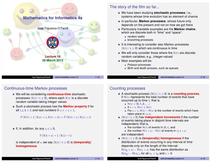
The story of the film so far... We have been studying stochastic processes ; i.e., systems whose time evolution has an element of chance Mathematics for Informatics 4a In particular, Markov processes , whose future only depends on the present and not on how we got there José Figueroa-O’Farrill Particularly tractable examples are the Markov chains , which are discrete both in “time” and “space”: random walks branching processes It is interesting to consider also Markov processes { X ( t ) | t � 0 } which are continuous in time We will only consider those where the X ( t ) are discrete Lecture 19 random variables; e.g., integer-valued 28 March 2012 Main examples will be: Poisson processes Birth and death process, such as queues José Figueroa-O’Farrill mi4a (Probability) Lecture 19 1 / 18 José Figueroa-O’Farrill mi4a (Probability) Lecture 19 2 / 18 Continuous-time Markov processes Counting processes A stochastic process { N ( t ) | t � 0 } is a counting process , We will be considering continuous-time stochastic if N ( t ) represents the total number of events that have processes { X ( t ) | t � 0 } , where each X ( t ) is a discrete occurred up to time t ; that is, random variable taking integer values N ( t ) ∈ { 0, 1, 2, . . . } Such a stochastic process has the Markov property if for If s < t , N ( s ) � N ( t ) all i , j , k ∈ Z and real numbers 0 � r < s < t , For s < t , N ( t ) − N ( s ) is the number of events which have taken place in ( s , t ] . P ( X ( t ) = j | X ( s ) = i , X ( r ) = k ) = P ( X ( t ) = j | X ( s ) = i ) { N ( t ) | t � 0 } has independent increments if the number of events taking place in disjoint time intervals are independent; that is, the number N ( t ) of events in [ 0, t ] , and If, in addition, for any s , t � 0, the number N ( t + s ) − N ( t ) of events in ( t , t + s ] are independent P ( X ( t + s ) = j | X ( s ) = i ) { N ( t ) | t � 0 } is (temporally) homogeneous if the distribution of events occurring in any interval of time is independent of s , we say { X ( t ) | t � 0 } is (temporally) depends only on the length of the interval: homogeneous N ( t 2 + s ) − N ( t 1 + s ) has the same distribution as N ( t 2 ) − N ( t 1 ) , for all t 1 < t 2 and s > 0 José Figueroa-O’Farrill mi4a (Probability) Lecture 19 3 / 18 José Figueroa-O’Farrill mi4a (Probability) Lecture 19 4 / 18

Poisson processes Inter-arrival times Let { N ( t ) | t � 0 } be a Poisson process with rate λ > 0 Definition Let T 1 be the time of the first event { N ( t ) | t � 0 } is Poisson with rate Let T n> 1 be the time between the ( n − 1 ) st and the n th λ > 0 if events N ( 0 ) = 0 { T 1 , T 2 , . . . } is the sequence of inter-arrival times P ( T 1 > t ) = P ( N ( t ) = 0 ) = e − λt , whence T 1 is exponentially it has independent increments distributed with mean 1 for all s , t � 0 and n ∈ N , λ The same is true for the other T n , e.g., P ( N ( s + t )− N ( s ) = n ) = e − λt ( λt ) n P ( T 2 > t | T 1 = s ) = P ( 0 events in ( s , s + t ] | T 1 = s ) n ! (indep. incr.) = P ( 0 events in ( s , s + t ]) (homogeneity) = P ( 0 events in ( 0, t ]) Since P ( N ( s + t ) − N ( s ) = n ) does not depend on s , = e − λt Poisson process are (temporally) homogeneous Hence, taking s = 0, one sees that N ( t ) is Poisson The { T n } for n � 1 are i.i.d. exponential random variables distributed with mean E ( N ( t )) = λt with mean 1 λ José Figueroa-O’Farrill mi4a (Probability) Lecture 19 5 / 18 José Figueroa-O’Farrill mi4a (Probability) Lecture 19 6 / 18 Waiting times Example The waiting time until the n th event ( n � 1) is Suppose that trains arrive at a station at a Poisson rate λ = 1 S n = � n per hour. i = 1 T i S n � t if and only if N ( t ) � n , whence What is the expected time until the 6th train arrives? 1 What is the probability that the elapsed time between the 2 ∞ ∞ e − λt ( λt ) j � � 6th and 7th trains exceeds 1 hour? P ( S n � t ) = P ( N ( t ) � n ) = P ( N ( t ) = j ) = j ! j = n j = n We are asked for E ( S 6 ) where S 6 is the waiting time until 1 the 6th train, hence E ( S 6 ) = 6 λ = 6 hours. Differentiating with respect to t , we get the probability We are asked for P ( T 7 > 1 ) = e − λ = e − 1 ≃ 37% 2 density function f S n ( t ) = λe − λt ( λt ) n − 1 ( n − 1 ) ! which is a “gamma” distribution E ( S n ) = � i E ( T i ) = n λ José Figueroa-O’Farrill mi4a (Probability) Lecture 19 7 / 18 José Figueroa-O’Farrill mi4a (Probability) Lecture 19 8 / 18

Time of occurrence is uniformly distributed Example (Stopping game) If we know that exactly one event has occurred by time t , Events occur according to a Poisson process { N ( t ) | t � 0 } with how is the time of occurrence distributed? rate λ . Each time an event occurs we must decide whether or not to stop, with our objective being to stop at the last event to For s � t , occur prior to some specified time τ . That is, if an event occurs P ( T 1 < s | N ( t ) = 1 ) = P ( T 1 < s and N ( t ) = 1 ) at time t , 0 < t < τ and we decide to stop, then we lose if there P ( N ( t ) = 1 ) are any events in the interval ( t , τ ] , and win otherwise. If we do = P ( N ( s ) = 1 and N ( t ) − N ( s ) = 0 ) not stop when an event occurs, and no additional events occur P ( N ( t ) = 1 ) by time τ , then we also lose. Consider the strategy that stops at = P ( N ( s ) = 1 ) P ( N ( t ) − N ( s ) = 0 ) the first event that occurs after some specified time s , 0 < s < τ . (indep. incr.) P ( N ( t ) = 1 ) What should s be to maximise the probability of winning? = λse − λs e − λ ( t − s ) We win if and only if there is precisely one event in ( s , τ ] , hence (homogeneity) λte − λt P ( � ) = P ( N ( τ ) − N ( s ) = 1 ) = e − λ ( τ − s ) λ ( τ − s ) = s t We differentiate with respect to s to find that the maximum λ , for which P ( � ) = e − 1 ≃ 37% occurs for s = τ − 1 i.e., it is uniformly distributed José Figueroa-O’Farrill mi4a (Probability) Lecture 19 9 / 18 José Figueroa-O’Farrill mi4a (Probability) Lecture 19 10 / 18 Example (Bus or walk?) Example (Bus or walk? — continued) Buses arrive to a stop according to a Poisson process Therefore, { N ( t ) | t � 0 } with rate λ . Your bus trip home takes b minutes E ( T ) = ( s + w ) e − λs + ( 1 λ + b )( 1 − e − λs ) from the time you get on the bus until you reach home. You can also walk home from the bus stop, the trip taking you w � � = 1 s + w − 1 e − λs λ + b + λ − b minutes. You adopt the following strategy: upon arriving at the bus stop, you wait for at most s minutes and start walking if no whose behaviour (as a function of s ) depends on the sign of bus has arrived by that time. (Otherwise you catch the first bus w − 1 λ − b . that comes.) Is there an optimal s which minimises the duration of your trip home? Let T denote the duration of the trip home from the time you arrive at the bus stop. Conditioning on the mode of transport, w − 1 w − 1 w − 1 λ − b < 0 λ − b = 0 λ − b > 0 E ( T ) = E ( T | N ( s ) = 0 ) P ( N ( s ) = 0 ) + E ( T | N ( s ) > 0 ) P ( N ( s ) > 0 ) The minimum is either at s = 0 (walk without waiting) or at = ( s + w ) e − λs + ( E ( T 1 ) + b )( 1 − e − λs ) s = ∞ (wait for the bus no matter how long) where T 1 is the first arrival time. Recall E ( T 1 ) = 1 λ . José Figueroa-O’Farrill mi4a (Probability) Lecture 19 11 / 18 José Figueroa-O’Farrill mi4a (Probability) Lecture 19 12 / 18