The story of the film so far... Partition rule: P ( A ) = P ( A | B ) - PowerPoint PPT Presentation

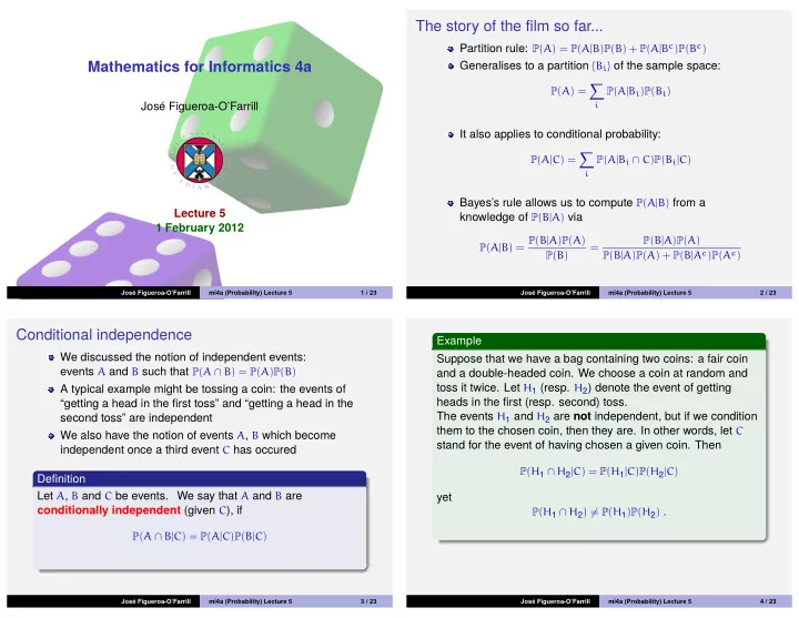
The story of the film so far... Partition rule: P ( A ) = P ( A | B ) P ( B ) + P ( A | B c ) P ( B c ) Mathematics for Informatics 4a Generalises to a partition { B i } of the sample space: � P ( A ) = P ( A | B i ) P ( B i ) Jos´ e Figueroa-O’Farrill i It also applies to conditional probability: � P ( A | C ) = P ( A | B i ∩ C ) P ( B i | C ) i Bayes’s rule allows us to compute P ( A | B ) from a Lecture 5 knowledge of P ( B | A ) via 1 February 2012 P ( A | B ) = P ( B | A ) P ( A ) P ( B | A ) P ( A ) = P ( B | A ) P ( A ) + P ( B | A c ) P ( A c ) P ( B ) Jos´ e Figueroa-O’Farrill mi4a (Probability) Lecture 5 1 / 23 Jos´ e Figueroa-O’Farrill mi4a (Probability) Lecture 5 2 / 23 Conditional independence Example We discussed the notion of independent events: Suppose that we have a bag containing two coins: a fair coin events A and B such that P ( A ∩ B ) = P ( A ) P ( B ) and a double-headed coin. We choose a coin at random and toss it twice. Let H 1 (resp. H 2 ) denote the event of getting A typical example might be tossing a coin: the events of heads in the first (resp. second) toss. “getting a head in the first toss” and “getting a head in the The events H 1 and H 2 are not independent, but if we condition second toss” are independent them to the chosen coin, then they are. In other words, let C We also have the notion of events A , B which become stand for the event of having chosen a given coin. Then independent once a third event C has occured P ( H 1 ∩ H 2 | C ) = P ( H 1 | C ) P ( H 2 | C ) Definition Let A , B and C be events. We say that A and B are yet conditionally independent (given C ), if P ( H 1 ∩ H 2 ) � = P ( H 1 ) P ( H 2 ) . P ( A ∩ B | C ) = P ( A | C ) P ( B | C ) Jos´ e Figueroa-O’Farrill mi4a (Probability) Lecture 5 3 / 23 Jos´ e Figueroa-O’Farrill mi4a (Probability) Lecture 5 4 / 23

Numerical outcomes Example (Continued) It is often the case that the outcomes of a trial are numbers or Indeed, by the partition rule and letting F denote the event of can be converted into numbers. having picked the fair coin, Notation P ( H 1 ∩ H 2 ) = P ( H 1 ∩ H 2 | F ) P ( F ) + P ( H 1 ∩ H 2 | F c ) P ( F c ) , We will denote such numerical outcomes by capital letters where P ( H 1 ∩ H 2 | F ) = 1 2 × 1 2 = 1 X , Y , ... and their values by lowercase x , y , .... 4 and P ( H 1 ∩ H 2 | F c ) = 1, whence Please observe this convention very carefully!!! P ( H 1 ∩ H 2 ) = ( 1 4 × 1 2 ) + ( 1 × 1 2 ) = 5 8 . Possible events now include On the other hand, the probability of getting a head is 3 4 since { Y > 0 } { a < X � b } { X = x } there are four faces in total, three of which are heads, whence and we will denote their probabilities by P ( H 1 ) P ( H 2 ) = 3 4 × 3 4 = 9 16 . P ( a < X � b ) P ( X = x ) P ( Y > 0 ) , respectively. Jos´ e Figueroa-O’Farrill mi4a (Probability) Lecture 5 5 / 23 Jos´ e Figueroa-O’Farrill mi4a (Probability) Lecture 5 6 / 23 Discrete probability distributions Example (Uniform distribution) Let us consider an experiment whose outcomes X are Generalising the above, we define the uniform distribution on integers. The probability distribution of X is the function { 1, 2, . . . , n } by p : Z → R defined by p ( x ) = P ( X = x ) for all x ∈ Z . It obeys 0 � p ( x ) � 1 and (see later) � � 1 x ∈ Z p ( x ) = 1. n , x ∈ { 1, 2, . . . , n } 1 p ( x ) = n · · · 0, otherwise Example (Dice) n 1 2 Consider rolling a fair die. The possible outcomes are Again notice that � , , . . . , , which we convert to a numerical outcome x ∈ Z p ( x ) = 1. X ∈ { 1, 2, . . . , 6 } in the obvious way. Then Example (Bernoulli trials) � 1 6 , x ∈ { 1, 2, 3, 4, 5, 6 } 1 Consider a Bernoulli trial with P ( S ) = p and P ( F ) = q = 1 − p . Let p ( x ) = 6 0, otherwise X ∈ { 0, 1 } denote the number of successes, so that p ( 0 ) = q and p ( 1 ) = p and p ( x ) = 0 for x � = 0, 1. Of course, � x ∈ Z p ( x ) = 1. 1 2 3 4 5 6 Notice that � x ∈ Z p ( x ) = 1. Jos´ e Figueroa-O’Farrill mi4a (Probability) Lecture 5 7 / 23 Jos´ e Figueroa-O’Farrill mi4a (Probability) Lecture 5 8 / 23

Example (Independent Bernoulli trials) Example (Binomial distribution) We could also consider a sequence of n independent Bernoulli Continuing with the previous example, it is clear that trials, each one with P ( S ) = p and P ( F ) = q = 1 − p . We let � � n p x q n − x , � x ∈ { 0, 1, . . . , n } X ∈ { 0, 1, . . . , n } denote the number of successes. x p ( x ) = 0, otherwise. X = 0 1 2 3 It is called the binomial distribution (with parameters n and 1 n = 0 p ). The quantity p ( x ) is the probability of getting exactly x successes in n trials. Notice that q p n = 1 n � n � � � p x q n − x = ( p + q ) n = 1 , p ( x ) = q 2 p 2 2 pq x n = 2 x ∈ Z x = 0 q 3 p 3 by the binomial theorem. n = 3 3 pq 2 3 p 2 q cf. Pascal’s triangle! Jos´ e Figueroa-O’Farrill mi4a (Probability) Lecture 5 9 / 23 Jos´ e Figueroa-O’Farrill mi4a (Probability) Lecture 5 10 / 23 Example (Tossing a fair coin) Example (The problem of the points) Suppose we toss a fair coin n times. This is just the previous In independent Bernoulli trials with success probability p , what example with p = q = 1 2 . Let X denote the number of heads. is the probability that n successes occur before m failures? Then This is the probability of there being at least n successes in � � n � 2 − n , 0 � x � n the first n + m − 1 trials. x p ( x ) = 0, otherwise. The probability of there being exactly k successes in n + m − 1 trials is given by the binomial distribution 0.5 0.5 0.4 0.4 � n + m − 1 � p k q n + m − 1 − k 0.3 0.3 k 0.2 0.2 0.1 0.1 Therefore the probability we are after is 0.30 0.25 n + m − 1 � � n + m − 1 � 0.20 p k q n + m − 1 − k 0.15 k k = n 0.10 0.05 � Jos´ e Figueroa-O’Farrill mi4a (Probability) Lecture 5 11 / 23 Jos´ e Figueroa-O’Farrill mi4a (Probability) Lecture 5 12 / 23 � � 0.15 0.15 � � 0.10 0.10 0.05 0.05 5 10 15 20

Example (Benford’s distribution) Example (Benford’s distribution – continued) Take any large collection of numerical data (e.g., census, It is actually very close to Benford’s distribution statistical tables, physical constants,...). What is the probability � log 10 ( 1 + 1 k ) , 1 � k � 9 distribution of the first significant digit? p ( k ) = For example, consider the sizes of files (in 512K blocks) in my 0, otherwise. laptop (excluding directories). It has over 2.5M files and the distribution of significant digits looks like this: 0.30 � 0.30 0.25 0.25 0.20 0.20 � 0.15 0.15 � 0.10 � 0.10 � � � 0.05 � � 0.05 Jos´ e Figueroa-O’Farrill mi4a (Probability) Lecture 5 13 / 23 Jos´ e Figueroa-O’Farrill mi4a (Probability) Lecture 5 14 / 23 Example (Benford’s distribution – continued) Example (Benford’s distribution under change of base) How about the distribution of the first two significant digits? Pulponio is an M-class planet, not unlike our own, whose Again, it is empirically very close to inhabitants count in base 8. Their chief scientist, Dr O. Fneb, observed empirically that the distribution of the most significant � log 10 ( 1 + 1 k ) , 10 � k � 99 digit in their statistical tables was very close to p ( k ) = 0, otherwise � log 8 ( 1 + 1 k ) , 1 � k � 7 p ( k ) = which is Benford’s 2-digit distribution . 0, otherwise. 99 Should this surprise us? It should not. In fact, if we take our � � log 10 ( 1 + 1 k + 1 p ( x ) = ) own statistical tables and re-express the entries in base b k k x ∈ Z k = 10 instead of base 10, we still get a distribution which is close to 99 � ( log 10 ( k + 1 ) − log 10 k ) = � log b ( 1 + 1 k ) , 1 � k � b − 1 k = 10 p ( k ) = 0, otherwise. = log 10 100 − log 10 10 = 1 Jos´ e Figueroa-O’Farrill mi4a (Probability) Lecture 5 15 / 23 Jos´ e Figueroa-O’Farrill mi4a (Probability) Lecture 5 16 / 23