The real story of the film so far... X a continuous random variable : - PowerPoint PPT Presentation

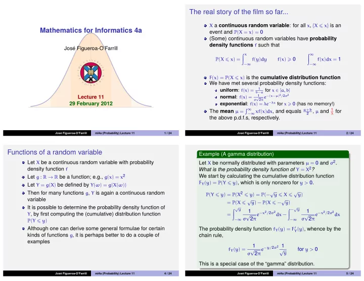
The real story of the film so far... X a continuous random variable : for all x , { X � x } is an Mathematics for Informatics 4a event and P ( X = x ) = 0 (Some) continuous random variables have probability density functions f such that Jos´ e Figueroa-O’Farrill � x � ∞ f ( x ) � 0 f ( x ) dx = 1 P ( X � x ) = f ( y ) dy − ∞ − ∞ F ( x ) = P ( X � x ) is the cumulative distribution function We have met several probability density functions: 1 uniform : f ( x ) = b − a for x ∈ [ a , b ] 2 π e −( x − µ ) 2 / 2 σ 2 1 Lecture 11 normal : f ( x ) = √ σ exponential : f ( x ) = λe − λx for x � 0 (has no memory!) 29 February 2012 � ∞ − ∞ xf ( x ) dx , and equals a + b 2 , µ and 1 The mean µ = λ for the above p.d.f.s, respectively. Jos´ e Figueroa-O’Farrill mi4a (Probability) Lecture 11 1 / 24 Jos´ e Figueroa-O’Farrill mi4a (Probability) Lecture 11 2 / 24 Functions of a random variable Example (A gamma distribution) Let X be normally distributed with parameters µ = 0 and σ 2 . Let X be a continuous random variable with probability density function f What is the probability density function of Y = X 2 ? We start by calculating the cumulative distribution function Let g : R → R be a function; e.g., g ( x ) = x 2 F Y ( y ) = P ( Y � y ) , which is only nonzero for y > 0. Let Y = g ( X ) be defined by Y ( ω ) = g ( X ( ω )) P ( Y � y ) = P ( X 2 � y ) = P (− √ y � X � √ y ) Then for many functions g , Y is again a continuous random variable = P ( X � √ y ) − P ( X � − √ y ) It is possible to determine the probability density function of � √ y � − √ y 1 1 e − x 2 / 2 σ 2 dx − e − x 2 / 2 σ 2 dx Y , by first computing the (cumulative) distribution function = √ √ 2 π 2 π σ σ − ∞ − ∞ P ( Y � y ) Although one can derive some general formulae for certain The probability density function f Y ( y ) = F ′ Y ( y ) , whence by the kinds of functions g , it is perhaps better to do a couple of chain rule, examples 1 e − y/ 2 σ 2 1 f Y ( y ) = for y > 0 √ √ y 2 π σ This is a special case of the “gamma” distribution. Jos´ e Figueroa-O’Farrill mi4a (Probability) Lecture 11 4 / 24 Jos´ e Figueroa-O’Farrill mi4a (Probability) Lecture 11 5 / 24

Expectation of a function of a random variable Example (The log-normal distribution) As before, X is a continuous random variable with Let X be normally distributed with parameters µ and σ 2 . What is probability density function f X the probability density function of Y = e X ? Then the expectation value E ( Y ) of Y = g ( X ) is given by Let us calculate P ( Y � y ) , which is only nonzero for y > 0. � ∞ P ( Y � y ) = P ( e X � y ) E ( Y ) = E ( g ( X )) = g ( x ) f ( x ) dx , − ∞ = P ( X � log y ) � log y (assuming the integral exists) 1 e −( x − µ ) 2 / 2 σ 2 dx = √ For example, σ 2 π − ∞ � ∞ E ( X 2 ) = x 2 f ( x ) dx whence − ∞ 1 e −( log y − µ ) 2 / 2 σ 2 1 and � ∞ f Y ( y ) = for y > 0 √ y E ( e tX ) = e tx f ( x ) dx 2 π σ − ∞ (provided the integrals exist) Jos´ e Figueroa-O’Farrill mi4a (Probability) Lecture 11 6 / 24 Jos´ e Figueroa-O’Farrill mi4a (Probability) Lecture 11 7 / 24 Variance of a continuous random variable Example (Variance of exponential distribution) Let X be a continuous random variables with mean µ = E ( X ) . Let X be exponentially distributed with parameter λ , so We define the variance of X by E ( X ) = 1 λ . Then Var ( X ) = E ( X 2 ) − µ 2 = E (( X − µ ) 2 ) � ∞ E ( X 2 ) = x 2 λe − λx dx The standard deviation is the (+ve) square-root of the 0 variance. � ∞ = λ d 2 e − λx dx Example (Variance of uniform distribution) dλ 2 0 Let X be uniformly distributed in [ a , b ] , so E ( X ) = 1 2 ( a + b ) . Then = λ d 2 1 λ = 2 dλ 2 λ 2 b � b � b 3 − a 3 3 x 3 1 x 2 � 3 ( a 2 + ab + b 2 ) E ( X 2 ) = = 1 = 1 b − adx = � whence 3 b − a b − a � Var ( X ) = E ( X 2 ) − µ 2 = 2 λ 2 − 1 λ 2 = 1 a � a λ 2 whence Var ( X ) = E ( X 2 ) − µ 2 = 1 3 ( a 2 + ab + b 2 ) − 1 4 ( a + b ) 2 = 1 12 ( a − b ) 2 Jos´ e Figueroa-O’Farrill mi4a (Probability) Lecture 11 8 / 24 Jos´ e Figueroa-O’Farrill mi4a (Probability) Lecture 11 9 / 24

Moment generating functions Example (Variance of normal distribution) Let X be a continuous random variable with probability density Let X be normally distributed with parameters µ = E ( X ) and σ . function f . The moment generating function (m.g.f.) M X ( t ) � ∞ is defined by 1 e −( x − µ ) 2 / 2 σ 2 dx Var ( X ) = E (( X − µ ) 2 ) = ( x − µ ) 2 √ � ∞ 2 π σ − ∞ M X ( t ) = E ( e tX ) = e tx f ( x ) dx � ∞ 1 y 2 e − y 2 / 2 σ 2 dy ( y = x − µ ) = − ∞ √ 2 π σ − ∞ (for those values of t for which the integral converges) � ∞ σ 2 u 2 e − u 2 / 2 du ( u = y/σ ) = √ Example (M.g.f. for uniform distribution) 2 π − ∞ � ∞ = − σ 2 Let X be uniformly distributed in [ a , b ] . Then u d due − u 2 / 2 du √ 2 π − ∞ � b b = e tb − e ta � d e tx e tx � � ∞ = − σ 2 � � M X ( t ) = b − adx = � ue − u 2 / 2 � − e − u 2 / 2 � du t ( b − a ) t ( b − a ) √ a � a du 2 π − ∞ 6 ( a 2 + ab + b 2 ) t 2 + · · · = 1 + 1 2 ( a + b ) t + 1 � ∞ σ 2 e − u 2 / 2 du = σ 2 = √ 2 π 3 ( a 2 + ab + b 2 ) , as − ∞ whence E ( X ) = 1 2 ( a + b ) and E ( X 2 ) = 1 computed earlier. Thus σ is the standard deviation. Jos´ e Figueroa-O’Farrill mi4a (Probability) Lecture 11 10 / 24 Jos´ e Figueroa-O’Farrill mi4a (Probability) Lecture 11 11 / 24 Example (M.g.f. for normal distribution) Example (M.g.f. for exponential distribution) Let X be normally distributed with mean µ and variance σ 2 . Let X be exponentially distributed with mean 1 λ . � ∞ 1 e tx e −( x − µ ) 2 / 2 σ 2 dx � ∞ M X ( t ) = √ e tx λe − λx dx M X ( t ) = 2 π σ − ∞ � ∞ 0 e tµ � ∞ e ty e − y 2 / 2 σ 2 dy = ( y = x − µ ) √ e −( λ − t ) x dx = λ 2 π σ − ∞ 0 � ∞ e tµ e −( y 2 − 2 σ 2 ty ) / 2 σ 2 dy λ = √ = 2 π σ − ∞ λ − t � ∞ = e tµ + 1 2 σ 2 t 2 1 e −( y − σ 2 t ) 2 / 2 σ 2 dy = √ 1 − t 2 π σ − ∞ λ � ∞ = e tµ + 1 2 σ 2 t 2 = 1 + 1 λt + 1 λ 2 t 2 + · · · e − u 2 / 2 σ 2 du ( u = y − σ 2 t ) √ 2 π σ − ∞ = e tµ + 1 2 σ 2 t 2 whence E ( X ) = 1 λ and E ( X 2 ) = 2 λ 2 as computed earlier. 2 ( σ 2 + µ 2 ) t 2 + · · · = 1 + µt + 1 2 ( µ 2 + σ 2 ) t 2 + · · · Notice that M X ( t ) = 1 + µt + 1 Jos´ e Figueroa-O’Farrill mi4a (Probability) Lecture 11 12 / 24 Jos´ e Figueroa-O’Farrill mi4a (Probability) Lecture 11 13 / 24

Some properties of mean and variance Standardising the normal distribution Theorem Theorem Let X be a continuous random variable. Then provided that Let X be normally distributed with parameters µ and σ . Then E ( X ) and E ( X 2 ) exist, we have for all a , b ∈ R , Y = 1 σ ( X − µ ) has as p.d.f. a standard normal distribution. E ( aX + b ) = a E ( X ) + b 1 Var ( aX + b ) = a 2 Var ( X ) 2 Remark It follows from the previous theorem that Y has mean Proof. E ( Y ) = 1 1 σ ( E ( X ) − µ ) = 0 and variance Var ( Y ) = σ 2 Var ( X ) = 1, follows by linearity of integration: 1 just like the standard normal distribution. Moreover the � ∞ � ∞ � ∞ moment generating function E ( aX + b ) = ( ax + b ) f ( x ) dx = a xf ( x ) dx + b f ( x ) dx 2 t 2 , − ∞ − ∞ − ∞ 1 M Y ( t ) = E ( e t ( X − µ ) /σ ) = e − µt/σ M X ( t σ ) = e = a E ( X ) + b which is the moment generating function of the standard normal distribution. This makes the theorem plausible, but we wish to follows from Var ( Y ) = E (( Y − µ Y ) 2 ) with Y = aX + b 2 prove it. Jos´ e Figueroa-O’Farrill mi4a (Probability) Lecture 11 14 / 24 Jos´ e Figueroa-O’Farrill mi4a (Probability) Lecture 11 15 / 24 Proof. Example (The standard error) We will instead show directly that Y has the cumulative Let X be normally distributed with mean µ and variance σ 2 . For distribution function of a standard normal distribution: which value of c > 0 is P ( | X − µ | � cσ ) = 0.5 ? This is the same c for which P ( | Y | � c ) = 0.5, where P ( Y � y ) = P ( 1 σ ( X − µ ) � y ) Y = 1 σ ( X − µ ) has a standard normal distribution: = P ( X � σy + µ ) � σy + µ � c 1 1 e −( x − µ ) 2 / 2 σ 2 dx e − y 2 / 2 dy = P ( | Y | � c ) = √ √ 2 π 2 π σ − ∞ − c � y � c 1 = 2 1 e − u 2 / 2 du e − y 2 / 2 dy ( u = 1 σ ( x − µ ) ) = √ √ 2 π 2 π 0 − ∞ � � c � 0 � = 2 1 e − y 2 / 2 dy whence P ( Y � y ) = Φ ( y ) . − √ 2 π − ∞ − ∞ The usefulness of this result is that if X is normally distributed, = 2 Φ ( c ) − 1 P ( | X − µ | � cσ ) = P ( | Y | � c ) Therefore P ( | Y | � c ) = 0.5 if and only if Φ ( c ) = 0.75. where c > 0 is some constant and Y = 1 σ ( X − µ ) . Jos´ e Figueroa-O’Farrill mi4a (Probability) Lecture 11 16 / 24 Jos´ e Figueroa-O’Farrill mi4a (Probability) Lecture 11 17 / 24