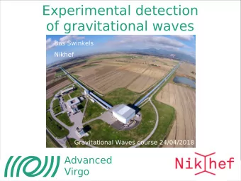
The Quest for Gravitational Waves 26/2/2016 B.A. Boom & L. van - - PowerPoint PPT Presentation

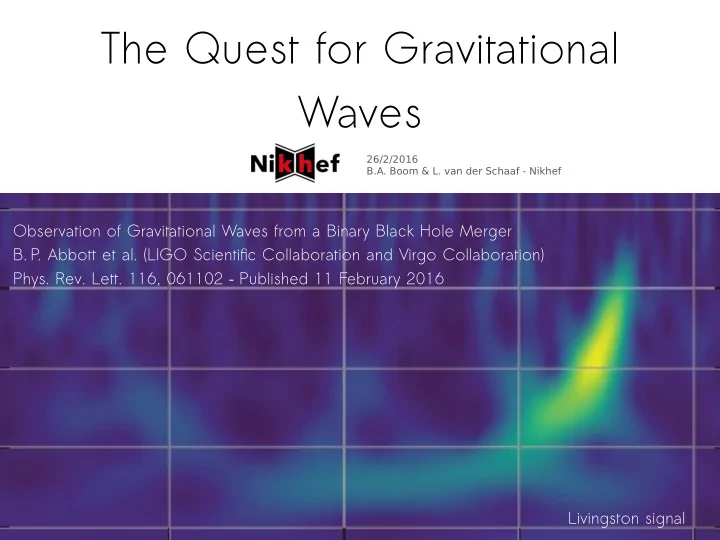
The Quest for Gravitational Waves

Finally we know we work on something real Laura

Observation of Gravitational Waves from a Binary Black Hole Merger

• B. P. Abbott et al. (LIGO Scientifc Collaboration and Virgo Collaboration)
• Phys. Rev. Lett. 116, 061102 – Published 11 February 2016

Livingston signal

26/2/2016 B.A. Boom & L. van der Schaaf - Nikhef

45 minutes to catch up on the work

• f 100 years:
• A brief History
• How do we measure gravitational waves?
• How do we now it is gravitational waves?
• What do these waves tell us?
• The future of gravitational waves

Gravitation

• Newton’s Theory of Gravity (1687)

Gravitation is an interaction force between masses This force is instantaneous

• Einstein’s Theory of Special Relativity (1905)

Laws of nature are the same for all inertial observers Light travels at the same speed according to all observers

➢

Close relationship between space and time (“spacetime”)

➢

Information can travel at most with the speed of light Where does gravity ft in this view?

Gravitation

• Newton’s Theory of Gravity (1687)

Gravitation is an interaction force between masses This force is instantaneous

• Einstein’s Theory of Special Relativity (1905)

Laws of nature are the same for all inertial observers Light travels at the same speed according to all observers

➢

Close relationship between space and time (“spacetime”)

➢

Information can travel at most with the speed of light Where does gravity ft in this view?

• Einstein’s Theory of General Relativity (1915)

Inertial observers in curved spacetime Matter causes this curvature Gravity is a side efgect of this curvature

Curved Light Paths

Curved Light Paths in experiment

New York Times, November 10, 1919

Sir Arthur Eddington

Dynamics: Gravitational Waves

GW time L-D L L+ D L

GW’s follow from general relativity

Waves in spacetime itself Coupling is very weak

1 1 2 44

10

− − −

m kg s

GW150914

• Gravitational wave observed in 2 detectors 3000 km

apart

• Binary black hole inspiral, merger and ringdown visible
• Maximum strain amplitude of 10-21!!!

Gravitational Wave Detectors

Tabletop “Gravitational Wave Detector”

• Michelson Interferometer
• Very sensitive to

difgerential arm change

• Strain sensitivity ~10-9

How Small is 10-21 Really?

The Real Thing

Beam splitter

Mirror: diameter 350 mm

Mechanical polishing tot 2 nm rms Ion-beam polishing tot 0.5 nm Corrective coating to 0.3 nm over 150 mm

Vibration Isolation

• Passive isolation based on pendulums
• Cascading will give very steep transfers

Resulting Sensitivity

Data analysis

All about gaining as much informationas possible

• With one source:
• Detect signals
• Estimate parameters: what source? Where?

With several sources:

• Study populations (astrophysics)
• Cosmology (cosmic distance ladder and primordial

gravitational waves)

Observation

Raw data GW150914

Get the data at: https://losc.ligo.org/events/GW150914/

Extracting the signal from the raw data

• Transient searches (arXiv:1602.03843v1)

– Made for short duration transients ( ~ ms to 10 s) – Depend little on the signal morphology

• Matched fltering (arXiv:1602.03839v1)

– Optimized for binary coalescence searches

Coherent WaveBurst (cWB)

• Low-latency pipeline (report of The Event with 3 min delay)
• Time-frequency analysis: Fourier transform with a window function
• Cross-correlation of the two detectors
• Classifcation: check that it does not fall in a glitch class, check some characteristic

source features

• Estimate sky location and wave polarization

Hanford time frequency The Event

Situation after this frst search

Ec is the dimensionless coherent signal energy obtained by cross- correlating the two reconstructed waveforms, and En is the dimensionless residual noise energy after the reconstructed signal is subtracted from the data. C1: known noise C2: remaining events C3: frequency increases with time

Defnition of cross-correlation:

Coherence of signals:

PyCBC: matched fltering

First consider an intuitive filter: strain = noise + signal : Not what is happening This is what is done Define a detection statistic: Refine the filter: Matched filter signal to noise and chi-squared: where Recomputed every 2084 s

PyCBC: matched fltering

Best ftting template

Situation after second test

Why are there numbers below 1?

The two test discussed are responsible to make detections: afterwards the parameters

• f the event are properly reconstructed (with Monte Carlo methods and nested

sampling algorithm).

Background estimation

• Background reduced by monitoring environment:

“seismometers, accelerometers, microphones, magnetometers, radio receivers, weather, sensors, ac-power line monitors and a cosmic-ray detector”

• Uncorrelated residual background estimated with time sliding
• Event 10^6 time slides
• Sliding by 10 ms => larger than GW travel time to get

uncorrelated noise

The signal after ftting to waveform models

36 +5/-4 Msun 29 + 4 Msun Final mass = 62 + 4 Msun Final spin = 0.67 +0.05/-0.07 410 +160/-180 Mpc or 0.09 +0.03/-0.04 in redshift

A wonderful chance to test GR!

Predict parameters and compare

QNM frequency of black hole

Deviations from best ft waveform

More on deviations

GR performed very well in this test ...

Graviton wavelength bound

By using: and

Future

• More detectors (Advanced Virgo, Kagra,

LigoIndia)

• More (diverse) sources (neutron stars,

black holes, supernovas, primordial gravitational waves, … ? )

• Difgerent types of detectors (ET, eLISA)