The Prominence of Stabilization Techniques in Column Generation: the - - PowerPoint PPT Presentation

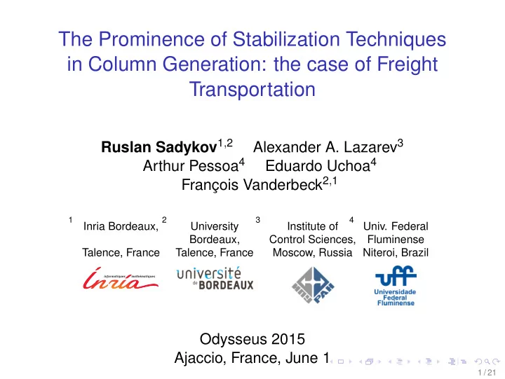
The Prominence of Stabilization Techniques in Column Generation: the case of Freight Transportation

Ruslan Sadykov1,2 Alexander A. Lazarev3 Arthur Pessoa4 Eduardo Uchoa4 François Vanderbeck2,1

1

Inria Bordeaux, Talence, France

2

University Bordeaux, Talence, France

3

Institute of Control Sciences, Moscow, Russia

4

• Univ. Federal

Fluminense Niteroi, Brazil

Odysseus 2015 Ajaccio, France, June 1

1 / 21

Contents

Freight railcar routing application Column generation approach Stabilization Results and conclusions

2 / 21

The freight car routing application: overview

initial car distribution transportation demands

3 / 21

Specificity of freight rail transportation in Russia

◮ Freight car

blocking

◮ Freight train

scheduling

◮ Locomotives

management

◮ Personnel

management The state company

◮ Assignment of

transportation demands to freight cars

◮ Freight car routing

Independent freight car management companies

• Transp. costs matrix
• Transp. times matrix

car movements

4 / 21

Specificity of freight rail transportation in Russia

◮ Freight car

blocking

◮ Freight train

scheduling

◮ Locomotives

management

◮ Personnel

management The state company

◮ Assignment of

transportation demands to freight cars

◮ Freight car routing

Independent freight car management companies

• Transp. costs matrix
• Transp. times matrix

car movements

Distances are large, and average freight train speed is low (≈ 300 km/day): discretization in periods of 1 day is reasonable

4 / 21

The freight car routing application: input and output

Input

◮ Railroad network (stations) ◮ Initial location of cars (sources) ◮ Transportation demands and associated profits ◮ Transportation times between stations ◮ Costs: transfer costs and standing (waiting) daily rates;

5 / 21

The freight car routing application: input and output

Input

◮ Railroad network (stations) ◮ Initial location of cars (sources) ◮ Transportation demands and associated profits ◮ Transportation times between stations ◮ Costs: transfer costs and standing (waiting) daily rates;

Output: operational plan

◮ A set of accepted demands and their execution dates ◮ Empty and loaded cars movements to meet the demands

(car routing)

Objective

Maximize the total net profit

5 / 21

Similar applications in the literature

[Fukasawa et al., 2002]

◮ Train schedule is known ◮ Cars should be assigned to trains to be transported ◮ Discretization by the moments of arrival and departure of

trains.

◮ Smaller time horizon (7 days)

6 / 21

Similar applications in the literature

[Fukasawa et al., 2002]

◮ Train schedule is known ◮ Cars should be assigned to trains to be transported ◮ Discretization by the moments of arrival and departure of

trains.

◮ Smaller time horizon (7 days)

Other works

◮ [Holmberg et al., 1998] ◮ [Löbel, 1998] ◮ [Lulli et al., 2011] ◮ [Caprara et al., 2011]

6 / 21

Commodity graph [Stratonnikov and Shiryaev, 2012]

Commodity c ∈ C represents the flow (movements) of cars of type c.

Graph Gc = (Vc, Ac) for commodity c ∈ C:

· · · · · · · · · station 1 station 2 station 3 · · · · · · · · · · · · · · · · · · · · · · · · waiting arc empty transfer arc loaded transfer arc time

Each vertex v ∈ Vc represent location of cars of type c on a certain station at a certain time standing at a certain rate ga — cost of arc a ∈ Ac

7 / 21

Multi-commodity flow formulation

Notations

Q — set of demands, Cq — set of car types compatible with demand q ∈ Q, nmax

q

— maximum number of cars to assign to demand q ∈ Q,

• nc

v — number of cars of type c situated initially in vertex v ∈ V.

Variables

xc

a ∈ Z+ — flow size along arc a ∈ Ac, c ∈ C

8 / 21

Multi-commodity flow formulation

Notations

Q — set of demands, Cq — set of car types compatible with demand q ∈ Q, nmax

q

— maximum number of cars to assign to demand q ∈ Q,

• nc

v — number of cars of type c situated initially in vertex v ∈ V.

Variables

xc

a ∈ Z+ — flow size along arc a ∈ Ac, c ∈ C

min

• c∈C
• a∈Ac

gaxc

a

• c∈Cq
• a∈Acq

xc

a ≤ nmax q

∀q ∈ Q

• a∈δ−(v)

xc

a −

• a∈δ+(v)

xc

a =

nc

v

∀c ∈ C, v ∈ Vc xc

a ∈ Z+

∀c ∈ C, a ∈ Vc

8 / 21

Contents

Freight railcar routing application Column generation approach Stabilization Results and conclusions

9 / 21

Path reformulation

◮ Sc — set of type c car “sources” = {v ∈ Vc :

nv > 0})

◮ Pc s — set of paths (type c car routes) from source s ∈ Sc

Variables

◮ λp — flow size along path p ∈ Pc s , s ∈ Sc, c ∈ C

min

• c∈C
• s∈Sc
• p∈Ps

gpath

p

λp

• c∈Cq
• s∈Sc
• p∈Pc

s : q∈Qpath p

λp ≤ nmax

q

∀q ∈ Q

• p∈Pc

s

λp = nc

s

∀c ∈ C, s ∈ Sc λp ∈ Z+ ∀c ∈ C, s ∈ Sc, p ∈ Pc

s

10 / 21

Column generation for path reformulation

◮ Pricing problem decomposes to shortest path problems,

• ne for each source

◮ slow: number of sources are thousands 11 / 21

Column generation for path reformulation

◮ Pricing problem decomposes to shortest path problems,

• ne for each source

◮ slow: number of sources are thousands

◮ To accelerate, for each c ∈ C, we search for an in-tree of

shortest paths to the terminal vertex from all s ∈ Sc

◮ drawback: some demands are severely “overcovered”, bad

convergence

11 / 21

Column generation for path reformulation

◮ Pricing problem decomposes to shortest path problems,

• ne for each source

◮ slow: number of sources are thousands

◮ To accelerate, for each c ∈ C, we search for an in-tree of

shortest paths to the terminal vertex from all s ∈ Sc

◮ drawback: some demands are severely “overcovered”, bad

convergence

◮ We developed an iterative procedure:

repeat Find an in-tree T from all non-exhausted sources; foreach path p in T in the order of its reduced cost do Find n′ — the maximum number of cars able to follow p; if n′ > 0 then Add λp to the restricted master; Reduce by n′ the number of cars in the source of p; Reduce by n′ the volume of all demands covered by p; until iteration limit k or all demands are covered or all sources are exhausted;

11 / 21

Diving Heuristic

Master problem solution λ∗ can be fractional, so we apply the diving heuristic [Joncour et al., 2010]

◮ use Depth-First Search ◮ at each node of the tree

◮ select least fractional column ¯

λp : rounded value ⌈¯ λp⌋ > 0

◮ add ⌈¯

λp⌋ to the partial solution

◮ update right-hand-side of the

master constraints

◮ apply preprocessing, which may

lead to a change in the pricing problem variables bounds

◮ solve the updated master LP 12 / 21

Contents

Freight railcar routing application Column generation approach Stabilization Results and conclusions

13 / 21

Column generation in the dual space

L(π) — Lagrangian dual function π η L(π) (πt, ηt) Outer approximation

14 / 21

Column generation in the dual space

L(π) — Lagrangian dual function π η L(π) (πt, ηt) Outer approximation

14 / 21

Column generation in the dual space

L(π) — Lagrangian dual function π η L(π) (πt, ηt) Outer approximation (ˆ π, ˆ L) π η L(π) Inner approximation

14 / 21

Dual Price Smoothing [Wentges, 1997]

˜ πt = αˆ π + (1 − α)πt (πin, ηin) := (ˆ π, ˆ L) (πout, ηout) := (πt, ηt) (πsep, ηsep) := α (πin, ηin) + (1 − α) (πout, ηout)

OUT SEP IN OUT SEP IN

15 / 21

Auto-adaptative α-schedule [Pessoa et al., 2014]

L ( π ) = ˆ L πin πout ˜ π g(˜ π)

decrease α increase α

16 / 21

Penalty functions [du Merle et al., 1999]

πt = argmax

π∈Rm

+

• Lt(π) − ˆ

St(π)

• L(π)

−ˆ S(π − ˆ π) (ˆ π, ˆ L)

πq ˆ Sq(πq − ˆ πq) ˆ π

∆ γ = 0.9 · nmax

q

Here: ∆ =

• q∈Q |π1

q − ˆ

π0

q|

|Q| · κ

17 / 21

Contents

Freight railcar routing application Column generation approach Stabilization Results and conclusions

18 / 21

Stabilization results

Real-life instances: 40-140 days horizon, 1,025 stations, up to 5,300 demands, 11 car types, 12,651 cars, and 8,232 sources. Up to ≈ 230 thousands nodes and 7.5 millions arcs.

19 / 21

Stabilization results

Real-life instances: 40-140 days horizon, 1,025 stations, up to 5,300 demands, 11 car types, 12,651 cars, and 8,232 sources. Up to ≈ 230 thousands nodes and 7.5 millions arcs.

40 60 80 100 120 140 1m 10m 1h 10h planning horizon length, days solution time (log scale)

No stabilization Smoothing stabilization

• Pen. func. stabilization (κ = 0.05)

Combined stabilization (κ = 0.1) size CG Smooth Pen Comb 40 23 19 32 21 60 117 73 155 95 80 570 234 178 114 100 2481 607 278 152 120 8947 1465 410 213 140 28884 3069 756 338

19 / 21

Diving heuristic results

All instances solved to optimality by the diving heuristic.

(means Lagrangian bound is equal to the optimal solution value).

20 / 21

Diving heuristic results

All instances solved to optimality by the diving heuristic.

(means Lagrangian bound is equal to the optimal solution value).

40 60 80 100 120 140 1m 5m 10m 15m 20m planning horizon length, days solution time

Column generation Column generation + diving Cplex 12.4 size CG +Diving Cplex 40 21 22 51 60 95 100 111 80 114 145 245 100 152 211 408 120 213 344 633 140 338 377 1127

20 / 21

Conclusions

◮ A freight car routing application can be modelled as the

multi-commodity flow problem

◮ Non-stabilized column generation implementation is not

competitive with Cplex

◮ Generic combined stabilization with a single parameter

gives up to 85x speed-up

◮ Generic diving heuristic allows us to obtain optimal integer

solutions for real-life instances up to 3 times faster than Cplex.

◮ Column-and-row generation [Sadykov et al., 2013] gives

better results that the stabilized column generation, but the diving heuristic cannot be directly applied

21 / 21

References I

Caprara, A., Malaguti, E., and Toth, P . (2011). A freight service design problem for a railway corridor. Transportation Science, 45(2):147–162. du Merle, O., Villeneuve, D., Desrosiers, J., and Hansen, P . (1999). Stabilized column generation. Discrete Mathematics, 194(1-3):229–237. Fukasawa, R., de Aragão, M. P ., Porto, O., and Uchoa, E. (2002). Solving the freight car flow problem to optimality. Electronic Notes in Theoretical Computer Science, 66(6):42 – 52. Holmberg, K., Joborn, M., and Lundgren, J. T. (1998). Improved empty freight car distribution. Transportation Science, 32(2):163–173. Joncour, C., Michel, S., Sadykov, R., Sverdlov, D., and Vanderbeck, F . (2010). Column generation based primal heuristics. Electronic Notes in Discrete Mathematics, 36:695 – 702. Löbel, A. (1998). Vehicle scheduling in public transit and lagrangean pricing. Management Science, 44(12):1637–1649.

22 / 21

References II

Lulli, G., Pietropaoli, U., and Ricciardi, N. (2011). Service network design for freight railway transportation: the italian case. Journal of the Operational Research Society, 62(12):2107–2119. Pessoa, A., Sadykov, R., Uchoa, E., and Vanderbeck, F. (2014). Automation and combination of linear-programming based stabilization techniques in column generation. Technical Report hal-01077984, HAL Inria, https://hal.inria.fr/hal-01077984. Sadykov, R., Lazarev, A. A., Shiryaev, V., and Stratonnikov, A. (2013). Solving a freight railcar flow problem arising in russia. In Frigioni, D. and Stiller, S., editors, 13th Workshop on Algorithmic Approaches for Transportation Modelling, Optimization, and Systems, volume 33 of OpenAccess Series in Informatics (OASIcs), pages 55–67, Dagstuhl, Germany. Schloss Dagstuhl–Leibniz-Zentrum fuer Informatik. Stratonnikov, A. and Shiryaev, V. (2012). A large-scale linear programming formulation for railcars flow management (in Russian). In Fifth Russian conference on Optimization Problems and Economic Applications, Omsk, Russia. Wentges, P . (1997). Weighted dantzig–wolfe decomposition for linear mixed-integer programming. International Transactions in Operational Research, 4(2):151–162.

23 / 21