The necessity and formulation of a robust (imprecise) Bayes Factor - PowerPoint PPT Presentation
The necessity and formulation of a robust (imprecise) Bayes Factor Patrick Schwaferts Ludwig-Maximilians-Universit at M unchen 01. August 2018 Patrick Schwaferts (LMU) Imprecise Bayes Factor 01. August 2018 1 / 18 Introduction
The necessity and formulation of a robust (imprecise) Bayes Factor Patrick Schwaferts Ludwig-Maximilians-Universit¨ at M¨ unchen 01. August 2018 Patrick Schwaferts (LMU) Imprecise Bayes Factor 01. August 2018 1 / 18
Introduction Patrick Schwaferts (LMU) Imprecise Bayes Factor 01. August 2018 2 / 18
Introduction Reproducibility crisis in psychological research Patrick Schwaferts (LMU) Imprecise Bayes Factor 01. August 2018 2 / 18
Introduction Reproducibility crisis in psychological research Rise of popularity of Bayesian Statistics: promoted as being the solution Patrick Schwaferts (LMU) Imprecise Bayes Factor 01. August 2018 2 / 18
Introduction Reproducibility crisis in psychological research Rise of popularity of Bayesian Statistics: promoted as being the solution Bayes Factor for comparing two hypotheses (“Bayesian t -Test”) Patrick Schwaferts (LMU) Imprecise Bayes Factor 01. August 2018 2 / 18
What is the Bayes Factor? Patrick Schwaferts (LMU) Imprecise Bayes Factor 01. August 2018 3 / 18
What is the Bayes Factor? Informal: A generalization of the Likelihood Ratio to include prior information. Patrick Schwaferts (LMU) Imprecise Bayes Factor 01. August 2018 3 / 18
From Likelihood Ratio to Bayes Factor I Patrick Schwaferts (LMU) Imprecise Bayes Factor 01. August 2018 4 / 18
From Likelihood Ratio to Bayes Factor I Situation: Two independent groups with observations x i and y j and model X i ∼ N ( µ, σ 2 ) , i = 1 , ..., n , Y j ∼ N ( µ + α, σ 2 ) , j = 1 , ..., m , with parameters µ , σ 2 , δ = α/σ . Patrick Schwaferts (LMU) Imprecise Bayes Factor 01. August 2018 4 / 18
From Likelihood Ratio to Bayes Factor I Situation: Two independent groups with observations x i and y j and model X i ∼ N ( µ, σ 2 ) , i = 1 , ..., n , Y j ∼ N ( µ + α, σ 2 ) , j = 1 , ..., m , with parameters µ , σ 2 , δ = α/σ . Research Question: Is there a difference between both groups? Patrick Schwaferts (LMU) Imprecise Bayes Factor 01. August 2018 4 / 18
From Likelihood Ratio to Bayes Factor I Situation: Two independent groups with observations x i and y j and model X i ∼ N ( µ, σ 2 ) , i = 1 , ..., n , Y j ∼ N ( µ + α, σ 2 ) , j = 1 , ..., m , with parameters µ , σ 2 , δ = α/σ . Research Question: Is there a difference between both groups? Hypotheses: H 0 : δ = 0 vs . H 1 : δ � = 0 Patrick Schwaferts (LMU) Imprecise Bayes Factor 01. August 2018 4 / 18
From Likelihood Ratio to Bayes Factor II Likelihood Ratio: µ,σ 2 ,δ f ( data | µ, σ 2 , δ ) max R 10 = L µ,σ 2 f ( data | µ, σ 2 , δ = 0) max Patrick Schwaferts (LMU) Imprecise Bayes Factor 01. August 2018 5 / 18
From Likelihood Ratio to Bayes Factor II Likelihood Ratio: µ,σ 2 ,δ f ( data | µ, σ 2 , δ ) max R 10 = L µ,σ 2 f ( data | µ, σ 2 , δ = 0) max Law of Likelihood: The extent to which the data support one model over another (:= evidence ) is equal to the ratio of their likelihoods. Patrick Schwaferts (LMU) Imprecise Bayes Factor 01. August 2018 5 / 18
From Likelihood Ratio to Bayes Factor II Likelihood Ratio: µ,σ 2 ,δ f ( data | µ, σ 2 , δ ) max R 10 = L µ,σ 2 f ( data | µ, σ 2 , δ = 0) max Law of Likelihood: The extent to which the data support one model over another (:= evidence ) is equal to the ratio of their likelihoods. Interpretation of LR: R 10 times as much evidence for the model chosen ( ∗ ) under H 1 The data is L than for the model chosen ( ∗ ) under H 0 . ( ∗ ) : chosen refers to the max -operation ⇒ L R 10 quantifies the maximum evidence for H 1 (in a comparison with H 0 ) Patrick Schwaferts (LMU) Imprecise Bayes Factor 01. August 2018 5 / 18
From Likelihood Ratio to Bayes Factor III Introducing Prior Probabilities: P ( H 1 ) P ( H 0 ) and Patrick Schwaferts (LMU) Imprecise Bayes Factor 01. August 2018 6 / 18
From Likelihood Ratio to Bayes Factor III Introducing Prior Probabilities: P ( H 1 ) P ( H 0 ) and Bayes Rule: P ( H 1 | data ) R 10 · P ( H 1 ) = L P ( H 0 | data ) P ( H 0 ) � �� � � �� � PosteriorOdds PriorOdds The data is used to learn about P ( H 1 ) and P ( H 0 ). Patrick Schwaferts (LMU) Imprecise Bayes Factor 01. August 2018 6 / 18
From Likelihood Ratio to Bayes Factor III Introducing Prior Probabilities: P ( H 1 ) P ( H 0 ) and Bayes Rule: P ( H 1 | data ) R 10 · P ( H 1 ) = L P ( H 0 | data ) P ( H 0 ) � �� � � �� � PosteriorOdds PriorOdds The data is used to learn about P ( H 1 ) and P ( H 0 ). Interpretation of Posterior Probabilities: After seeing the data, the maximum belief in H 1 is P ( H 1 | data ). Patrick Schwaferts (LMU) Imprecise Bayes Factor 01. August 2018 6 / 18
From Likelihood Ratio to Bayes Factor IV Introducing Parameter Priors: P µ , P σ 2 and P δ Patrick Schwaferts (LMU) Imprecise Bayes Factor 01. August 2018 7 / 18
From Likelihood Ratio to Bayes Factor IV Introducing Parameter Priors: P µ , P σ 2 and P δ Bayesian Hypotheses: µ ∼ P µ µ ∼ P µ H B H B σ 2 ∼ P σ 2 σ 2 ∼ P σ 2 0 : vs . 1 : δ = 0 δ ∼ P δ P δ is called test-relevant prior . Patrick Schwaferts (LMU) Imprecise Bayes Factor 01. August 2018 7 / 18
From Likelihood Ratio to Bayes Factor IV Introducing Parameter Priors: P µ , P σ 2 and P δ Bayesian Hypotheses: µ ∼ P µ µ ∼ P µ H B H B σ 2 ∼ P σ 2 σ 2 ∼ P σ 2 0 : vs . 1 : δ = 0 δ ∼ P δ P δ is called test-relevant prior . Marginalized Likelihoods: ��� m ( data | H B f ( data | µ, σ 2 , δ ) P µ ( µ ) P σ 2 ( σ 2 ) P δ ( δ ) d δ d σ 2 d µ 1 ) = �� m ( data | H B f ( data | µ, σ 2 , δ = 0) P µ ( µ ) P σ 2 ( σ 2 ) d σ 2 d µ 0 ) = Patrick Schwaferts (LMU) Imprecise Bayes Factor 01. August 2018 7 / 18
From Likelihood Ratio to Bayes Factor V Bayes Factor: BF 10 = m ( data | H B 1 ) m ( data | H B 0 ) Patrick Schwaferts (LMU) Imprecise Bayes Factor 01. August 2018 8 / 18
From Likelihood Ratio to Bayes Factor V Bayes Factor: BF 10 = m ( data | H B 1 ) m ( data | H B 0 ) Bayes Rule: P ( H B 0 | data ) = BF 10 · P ( H B 1 | data ) 1 ) P ( H B P ( H B 0 ) The data is used to learn about P ( H B 1 ) and P ( H B 0 ). Nothing can be ⇒ P δ is part of the H B learned about the parameter priors. 1 -model. Patrick Schwaferts (LMU) Imprecise Bayes Factor 01. August 2018 8 / 18
From Likelihood Ratio to Bayes Factor V Bayes Factor: BF 10 = m ( data | H B 1 ) m ( data | H B 0 ) Bayes Rule: P ( H B 0 | data ) = BF 10 · P ( H B 1 | data ) 1 ) P ( H B P ( H B 0 ) The data is used to learn about P ( H B 1 ) and P ( H B 0 ). Nothing can be ⇒ P δ is part of the H B learned about the parameter priors. 1 -model. Interpretation of BF: The data is BF 10 times as much evidence for the model behind m ( data | H B 1 ) than for the model behind m ( data | H B 0 ) . Patrick Schwaferts (LMU) Imprecise Bayes Factor 01. August 2018 8 / 18
What is the model behind m ( data | H B 1 )? Patrick Schwaferts (LMU) Imprecise Bayes Factor 01. August 2018 9 / 18
What is the model behind m ( data | H B 1 )? Again Bayes Rule: 1 | data ) = m ( data | H B 1 ) · P ( H 1 ) P ( H B P ( data ) Patrick Schwaferts (LMU) Imprecise Bayes Factor 01. August 2018 9 / 18
What is the model behind m ( data | H B 1 )? Again Bayes Rule: 1 | data ) = m ( data | H B 1 ) · P ( H 1 ) P ( H B P ( data ) In order to apply Bayes Rule, m ( data | H B 1 ) needs to be a likelihood, which describes the data-generating process. Patrick Schwaferts (LMU) Imprecise Bayes Factor 01. August 2018 9 / 18
What is the model behind m ( data | H B 1 )? Again Bayes Rule: 1 | data ) = m ( data | H B 1 ) · P ( H 1 ) P ( H B P ( data ) In order to apply Bayes Rule, m ( data | H B 1 ) needs to be a likelihood, which describes the data-generating process. So the model behind m ( data | H B 1 ) models a data-generating process with likelihood ��� m ( data | H B f ( data | µ, σ 2 , δ ) P µ ( µ ) P σ 2 ( σ 2 ) P δ ( δ ) d δ d σ 2 d µ 1 ) = Patrick Schwaferts (LMU) Imprecise Bayes Factor 01. August 2018 9 / 18
What is the model behind m ( data | H B 1 )? Again Bayes Rule: 1 | data ) = m ( data | H B 1 ) · P ( H 1 ) P ( H B P ( data ) In order to apply Bayes Rule, m ( data | H B 1 ) needs to be a likelihood, which describes the data-generating process. So the model behind m ( data | H B 1 ) models a data-generating process with likelihood ��� m ( data | H B f ( data | µ, σ 2 , δ ) P µ ( µ ) P σ 2 ( σ 2 ) P δ ( δ ) d δ d σ 2 d µ 1 ) = ⇒ A model with subjective components! Patrick Schwaferts (LMU) Imprecise Bayes Factor 01. August 2018 9 / 18
What is the model behind m ( data | H B 1 )? Again Bayes Rule: 1 | data ) = m ( data | H B 1 ) · P ( H 1 ) P ( H B P ( data ) In order to apply Bayes Rule, m ( data | H B 1 ) needs to be a likelihood, which describes the data-generating process. So the model behind m ( data | H B 1 ) models a data-generating process with likelihood ��� m ( data | H B f ( data | µ, σ 2 , δ ) P µ ( µ ) P σ 2 ( σ 2 ) P δ ( δ ) d δ d σ 2 d µ 1 ) = ⇒ A model with subjective components! [The Bayes Factor does not directly answer: Is there an effect? ] Patrick Schwaferts (LMU) Imprecise Bayes Factor 01. August 2018 9 / 18
Necessity of properly specifying P δ Patrick Schwaferts (LMU) Imprecise Bayes Factor 01. August 2018 10 / 18
Recommend
More recommend
Explore More Topics
Stay informed with curated content and fresh updates.
