The Monte Carlo Method Estimating through sampling (estimating , p - PowerPoint PPT Presentation
The Monte Carlo Method Estimating through sampling (estimating , p -value, integrals,...) The main difficulty - sampling sparse events The general sampling to counting reduction The Markov Chain Monte Carlo (MCMC) method -
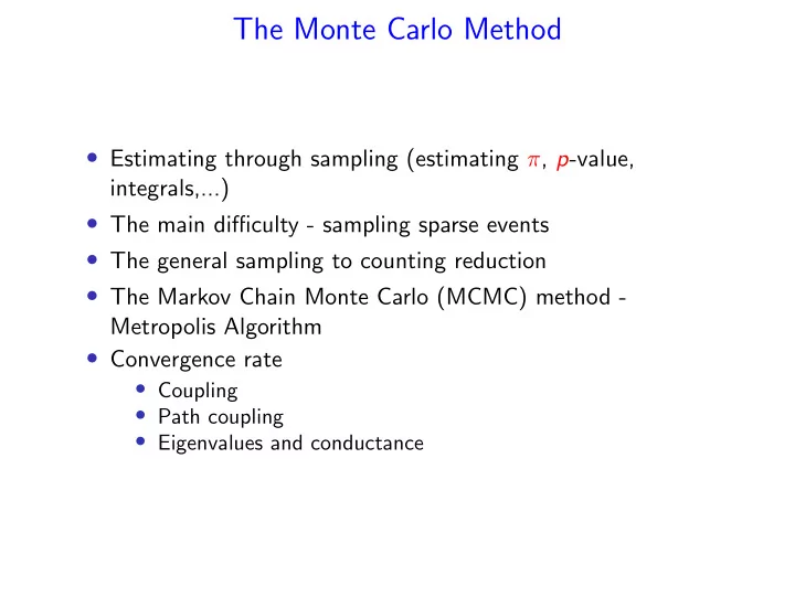
The Monte Carlo Method • Estimating through sampling (estimating π , p -value, integrals,...) • The main difficulty - sampling sparse events • The general sampling to counting reduction • The Markov Chain Monte Carlo (MCMC) method - Metropolis Algorithm • Convergence rate • Coupling • Path coupling • Eigenvalues and conductance
The Monte Carlo Method Example: estimate the value of π . 1 • Choose X and Y independently and uniformly at random in [0 , 1]. • Let √ X 2 + Y 2 ≤ 1 , � 1 if Z = 0 otherwise, • Pr( Z = 1) = π 4 . • 4 E [ Z ] = π .
• Let Z 1 , . . . , Z m be the values of m independent experiments. W = � m i =1 Z i . • � m m � E [ Z i ] = m π � � E [ W ] = E Z i = 4 , i =1 i =1 • W ′ = 4 m W is an unbiased estimate for π . • | W − m π 4 | ≥ ǫ m π Pr( | W ′ − π | ≥ ǫπ ) � � = Pr 4 Pr ( | W − E [ W ] | ≥ ǫ E [ W ]) = 2 e − 1 12 m πǫ 2 . ≤
( ǫ, δ )-Approximation Definition A randomized algorithm gives an ( ǫ, δ ) -approximation for the value V if the output X of the algorithm satisfies Pr( | X − V | ≤ ǫ V ) ≥ 1 − δ. Theorem Let X 1 , . . . , X m be independent and identically distributed indicator 3 ln 2 random variables, with µ = E [ X i ] . If m ≥ ǫ 2 µ , then δ �� m � � 1 � � � Pr X i − µ � ≥ ǫµ ≤ δ. � � � m � � i =1 That is, m samples provide an ( ǫ, δ ) -approximation for µ .
Monte Carlo Integration � b We want to compute the definite (numeric) integral a f ( x ) dx when the integral does not have a close form. Let a = x 0 , . . . , x N = b such that for all i , x i +1 − x i = b − a = δ ( N ). N � b N N b − a � � f ( x ) dx = lim f ( x i ) δ ( N ) = lim f ( x i ) . N N →∞ δ ( N ) → 0 a i =0 i =0 We need to estimate N 1 ¯ � f = lim f ( x i ) , N N →∞ i =0 which is the expected value of f () in [ a , b ].
We need to estimate N 1 ¯ � f = lim f ( x i ) . N N →∞ i =0 We choose N independent samples y 1 , . . . , y N uniformly distributed in [ a , b ]. N E [ 1 � f ( y i )] = ¯ f N i =1 N Var [ 1 f ( y i )] = 1 � N Var [ f ( x )] N i =1 N Pr ( | 1 f | ≥ ǫ ) ≤ Var [ f ( x )] � f ( y i ) − ¯ N ǫ 2 N i =1
Approximate Counting Example counting problems: 1 How many spanning trees in a graph? 2 How many perfect matchings in a graph? 3 How many independent sets in a graph? 4 ....
DNF Counting (Karp, Luby, Madras) DNF = Disjunctive Normal Form. Problem: How many satisfying assignments to a DNF formula? A DNF formula is a disjunction of clauses. Each clause is a conjunction of literals. ( x 1 ∧ x 2 ) ∨ ( x 2 ∧ x 3 ) ∨ ( x 1 ∧ x 2 ∧ x 3 ∧ x 4 ) ∨ ( x 3 ∧ x 4 ) Compare to CNF. ( x 1 ∨ x 2 ) ∧ ( x 1 ∨ x 3 ) ∧ · · · m clauses, n variables Let’s first convince ourselves that obvious approaches don’t work!
DNF counting is hard Question: Why? We can reduce CNF satisfiability to DNF counting. The negation of a CNF formula is in DNF. 1 CNF formula f 2 get the DNF formula (¯ f ) 3 count satisfying assignments to ¯ f 4 If it was 2 n , then f is unsatisfiable.
DNF counting is #P complete #P is the counting analog of NP. Any problem in #P can be reduced (in polynomial time) to the DNF counting problem. Example #P complete problems: 1 How many Hamilton circuits does a graph have? 2 How many satisfying assignments does a CNF formula have? 3 How many perfect matchings in a graph? What can we do about a hard problem?
( ǫ, δ ) FPRAS for DNF counting n variables, m clauses. FPRAS = “Fully Polynomial Randomized Approximation Scheme” Notation: U : set of all possible assignments to variables | U | = 2 n . H ⊂ U : set of satisfying assignments Want to estimate Y = | H | Give ǫ > 0 , δ > 0, find estimate X such that 1 Pr[ | X − Y | > ǫ Y ] < δ 2 Algorithm should be polynomial in 1 /ǫ , 1 /δ , n and m .
Monte Carlo method Here’s the obvious scheme. 1. Repeat N times: 1.1. Sample x randomly from U 1.2. Count a success if x ∈ H 2. Return “fraction of successes” × | U | . Question : How large should N be? We have to evaluate the probability of our estimate being good.
Let ρ = | H | | U | . Z i = 1 if i -th trial was successful � 1 with probability ρ Z i = 0 with probability 1 − ρ N � Z = Z i is a binomial r.v i =1 E [ Z ] = N ρ X = Z N | U | is our estimate of | H |
Probability that our algorithm succeeds Recall: X denotes our estimate of | H | . Pr[(1 − ǫ ) | H | < X < (1 + ǫ ) | H | ] Pr[(1 − ǫ ) | H | < Z | U | / N < (1 + ǫ ) | H | ] = = Pr[(1 − ǫ ) N ρ < Z < (1 + ǫ ) N ρ ] 1 − e − N ρǫ 2 / 3 − e − N ρǫ 2 / 2 > 1 − 2 e − N ρǫ 2 / 3 > where we have used Chernoff bounds. For an ( ǫ, δ ) approximation, this has to be greater than 1 − δ , 2 e − N ρǫ 2 / 3 < δ ρǫ 2 log 2 3 N > δ
Theorem Let ρ = | H | / | U | . Then the Monte Carlo method is an ( ǫ, δ ) approximation scheme for estimating | H | provided that ρǫ 2 log 2 3 N > δ .
What’s wrong? How large could 1 ρ be? ρ is the fraction of satisfying assignments. 1 The number of possible assignments is 2 n . 2 Maybe there are only a polynomial (in n ) number of satisfying assignments. 3 So, 1 ρ could be exponential in n . Question: An example where formula has only a few assignments?
The trick: Change the Sampling Space Increase the hit rate ( ρ )! Sample from a different universe, ρ is higher, and all elements of H still represented. What’s the new universe? Notation: H i set of assignments that satisfy clause i . H = H 1 ∪ H 2 ∪ . . . H m Define a new universe � � � U = H 1 H 2 . . . H m � means multiset union . Element of U is ( v , i ) where v is an assignment, i is the satisfied clause.
Example - Partition by clauses ( x 1 ∧ x 2 ) ∨ ( x 2 ∧ x 3 ) ∨ ( x 1 ∧ x 2 ∧ x 3 ∧ x 4 ) ∨ ( x 3 ∧ x 4 ) x 1 x 2 x 3 x 4 Clause 0 1 0 0 1 0 1 0 1 1 0 1 1 0 1 0 1 1 1 1 0 1 1 0 2 0 1 1 1 2 1 1 1 0 2 1 1 1 1 2 1 1 0 1 3 0 0 1 0 4 0 1 1 0 4
More about the universe U 1 Element of U is ( v , i ) where v is an assignment, i is the satisfied clause. 2 U contains only the satisfying assignments. 3 U contains the same satisfying assignment many times. U = { ( v , i ) | v ∈ H i } 4 Each satisfying assignment v appears in as many clauses as it satisfies.
One way of looking at U Partition by clauses. m partitions, partition i contains H i .
Another way of looking at U Partition by assignments (one region for each assignment v ). Each partition corresponds to an assignment. Can we count the different (distinct) assignments?
Example - Partition by assignments ( x 1 ∧ x 2 ) ∨ ( x 2 ∧ x 3 ) ∨ ( x 1 ∧ x 2 ∧ x 3 ∧ x 4 ) ∨ ( x 3 ∧ x 4 ) x 1 x 2 x 3 x 4 Clause 0 0 1 0 4 0 1 0 0 1 0 1 0 1 1 0 1 1 0 1 0 1 1 0 2 0 1 1 0 4 0 1 1 1 1 0 1 1 1 2 1 0 1 0 4 1 1 0 1 3 1 1 1 0 2 1 1 1 0 4
Canonical element Crucial idea: For each assignment group, find a canonical element in U . An element ( v , i ) is canonical if f (( v , i )) = 1 � 1 if i = min { j : v ∈ H j } f (( v , i )) = 0 otherwise For every assignment group, exactly one canonical element. So, count the number of canonical elements! Note: could use any other definition as long as exactly one canonical element per assignment
Count canonical elements Reiterating: 1 Number of satisfying assignments = Number of canonical elements. 2 Count number of canonical elements. 3 Back to old random sampling method for counting!
What is ρ ? Lemma ρ ≥ 1 m, (pretty large). Proof: | H | = | ∪ m i =1 H i | , since H is a normal union. So | H i | ≤ | H | � H 2 � . . . � H m Recall U = H 1 | U | = � m i =1 | H i | , since U is a multiset union. | U | ≤ m | H | ρ = | H | | U | ≥ 1 m
How to generate a random element in U ? Look at the partition of U by clauses. Algorithm Select: 1 Pick a random clause weighted according to the area it occupies. Pr[ i ] = | H i | | H i | | U | = � m 1 | H j | | H i | = 2 ( n − k i ) where k i is the number of literals in clause i . 2 Choose a random satisfying assignment in H i . • Fix the variables required by clause i . • Assign random values to the rest to get v ( v , i ) is the random element. Running time: O ( n ).
How to test if canonical assignment? Or how to evaluate f (( v , i ))? Algorithm Test: 1 Test every clause to see if v satisfies it. cov ( v ) = { ( v , j ) | v ∈ H j } 2 If ( v , i ) the smallest j in cov ( v ), then f ( v , i ) = 1, else 0. Running time: O ( nm ).
Back to random sampling Algorithm Coverage: 1 s ← 0 (number of successes) 2 Repeat N times: • Select ( v , i ) using Select . • if f ( v , i ) = 1 (check using Test ) then success, increment s . 3 Return s | U | / N . Number of samples needed is (from Theorem 4): ǫ 2 ρ ln 2 3 δ ≤ 3 m ǫ 2 ln 2 N = δ Sampling, testing: polynomial in n and m We have an FPRAS Theorem The Coverage algorithm yields an ( ǫ, δ ) approximation to | H | provided that the number of samples N ≥ 3 m ǫ 2 log 2 δ .
Size of Union of Sets Let H 1 , . . . , H k be subsets of a finite set S . What is the size of H = ∪ k i =1 H i ? Theorem The Coverage algorithm yields an ( ǫ, δ ) approximation to | H | provided that the number of samples N ≥ 3 k ǫ 2 log 2 δ .
Recommend
More recommend
Explore More Topics
Stay informed with curated content and fresh updates.

