The Minimum Spanning Tree Problem The Road to Linear Complexity - PowerPoint PPT Presentation
The Minimum Spanning Tree Problem The Road to Linear Complexity Marius-Florin Cristian Thesis supervisor: Jyrki Katajainen August 30, 2018 Content Overview Problem Definition and Goals General Overview Greedy Algorithms Non-greedy
The Minimum Spanning Tree Problem The Road to Linear Complexity Marius-Florin Cristian Thesis supervisor: Jyrki Katajainen August 30, 2018
Content Overview Problem Definition and Goals General Overview Greedy Algorithms Non-greedy Algorithms Developing ideas A classification of sparse graphs Trimming the subtrees of the graph A hierarchy of cycles A General Algorithm Reducing the density of the graph Improving the bottleneck of the disjoint sets Fighting the errors Conclusions The Road Developed Ideas Future Work
Overview ◮ Problem definition ◮ Goals of the thesis ◮ General overview of the road ◮ Greedy overview of the road ◮ Non-greedy overview of the road
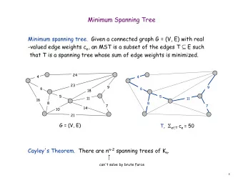
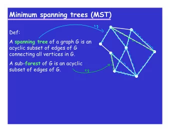
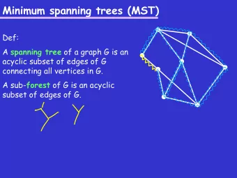
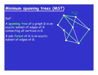
Problem Definition and Goals ◮ Problem Definition Given an undirected, connected graph G = ( V , E , C ), where V = { v 1 , v 2 , ... v n } is the vertex set, E = { e 1 , e 2 , ..., e m } the edge set, and each edge e i has a cost (or weight) associated c i ∈ C , where C = { c 1 , c 2 , ..., c m } . Let | V | = n and | E | = m . A spanning tree T = ( V , E ′ ) of G connects its vertices and the edge set E ′ ⊆ E has n − 1 edges. The weight of that spanning tree is the sum of the cost of its edges, i.e. � e i , j ∈ E ′ c i , j . In the minimum-spanning-tree problem the task is to find a spanning tree of G for which the cost is minimum. We do not allow duplicate edges.
Problem Definition and Goals ◮ Goals of the thesis. In order to solve the open problem, one must compute the minimum spanning tree of a given graph in a deterministic fashion in linear time with respect to the number of edges. This thesis explores the progress done until the current day and tries to solve the problem.
General Overview
Greedy Overview
Non-greedy Overview
Developing ideas ◮ A look at special cases of graphs ◮ Similarities between planar graphs and sparse graphs ◮ A classification of sparse graphs ◮ Trimming the subtrees of a graph ◮ A hierarchy of cycles
Graph structural properties ◮ The problem is not solved for general case graphs. ◮ The problem is solved for dense enough graphs. ◮ The problem is solved for planar graphs. ◮ The problem is NOT solved for sparse graphs with no apparent structural properties. How can we force structure to our graph?
Planar Graph properties One quickly notices that when dealing with a planar graph, the triangle inequality can be exploited in order to bound the neighbourhood of each point. A linear time algorithm follows just from the Delaunay triangulation of such a graph. The main property that a planar graph has in common with a general sparse graph is that the degree of each vertex under inspection is low. For a general sparse graph (number of edges < 4 n ) with vertices of low degree ( < 4), the problem should be solvable in linear time.
Classification of sparse graphs ◮ Sparse graphs with only low degree components We superficially argue that it should be possible to solve this case in a greedy fashion, either by applying one of the classical algorithms, or by detecting the cycles and trimming the trees. (more on this technique next) ◮ Sparse graphs with some high degree components High degree components are part of more cycles. If we use a greedy approach to keep track of the edges of such components we will end up with n edges, and the running time will be in a factor of n for just one such component.
Two types of sparse graphs
High degree sparse graph ◮ How shall we trim the vertices of degree 1? ◮ It can cascade in a succession of trims that could cover the whole graph ◮ What happens if there are more components of high degree?
High degree sparse graph ◮ How shall we trim the vertices of degree 1? An idea would be to keep track of the cycles from the shortest to the longest, and given a vertex of degree 1, to answer in constant time to which tree it belongs such that the root of the tree is a cycle. ◮ It can cascade in a succession of trims that could cover the whole graph We can avoid any such cascades by classifying such a hierarchy of cycles on levels, and then start the trimming process from the ”longest” cycle. First we remove the heaviest edge from each disjoint cycle on each level. ◮ What happens if there are more components of high degree?
Detecting cycles
Sparse graphs with mixed structure
A General Algorithm ◮ Reduce the density of the components such that cycle detection is easy ◮ The bottleneck will be the data structure used to detect cycles ◮ Disjoint Sets with table look-up ◮ Fighting the error produced by the disjoint sets
Density Reduction ◮ Reduce the density of the components such that cycle detection is easy Here we can artificially group components of high degree to cluster by applying Bor˚ uvka Phases, then apply the dense case algorithm to reduce the number of edges. The problem is more subtle, as we inspect only local components and we might discard good edges by doing such things. Thus we must consider the border edges as well.
Density Reduction When dealing with density reduction we must consider the following components: ◮ Components of high degree and high degree neighbours ◮ Components of high degree and low degree neighbours ◮ Components of high degree and mixed degree neighbours ◮ Components of low degree and high degree neighbours ◮ Components of low degree and low degree neighbours ◮ Components of low degree and mixed degree neighbours
Disjoint sets for cycle detection ◮ The disjoint sets data structure is good at detecting cycles ◮ We pick a vertex of high degree and find all of it’s closest cycles; Union-Find each of it’s neighbours, continue until a cycle is found. (example on blackboard) ◮ We mark the visited vertices and edges ◮ We pick an unmarked vertex of high degree and repeat the procedure The vertex will either form cycles with already marked ones, or new cycles. ◮ Such a pass will take O ( m + n ) time. Bounding the number of passes (blackboard). ◮ Each formed cycle is considered to be 1 vertex in future iterations We must also consider if during the density reduction a component had several expansions towards border edges.
Disjoint sets with table lookup ◮ The upper bound for disjoint set with union by rank and path compression is O ( m α ( m , n )) ◮ If we know the structure of unions in advance Gabow and Tarjan show that look-up tables can be computed for components of size Ω(log log n ) such that the running time of the disjoint sets will be O ( m + n ) ◮ We can approximate such a union structure, by expanding the dense components and computing the look-up tables ◮ Dense components are more likely to be part of more cycles
Disjoint sets with table lookup However two side effects might occur from using such a table look-up with the approximation of the union structure: ◮ The components are connected but the answer to a Find is false. A Union is usually performed, then the components will get connected again which will take O(1) time since there is nothing to do but try to connect. We can correct the value of the table in O(1) to properly reflect the component, and mark the Find as faulty; thus only after a Union we can check if the edge under inspection is part of a cycle or not. This should not worry us as there is no harm done.
Disjoint sets with table lookup ◮ The components are not connected and the answer to a Find is true, then the components will not get connected at this point in time. We might consider an edge as part of a cycle even if it isnt. This can create phantom cycles in the running of the algorithm. The phantom cycles can be addressed after the hierarchy of cycles has been established. The obvious side-effect is that some edges that are part of the MST might be omitted This should worry us as there is a lot of harm done. To counter this, we must either try to predict the structure of the MST pretty good, or aim in creating a pseudoforest, where we allow some cycles, and some disconnected components. (blackboard explanation)
Fighting the errors In order to fight the badness produced by the hardcoded tables we need to: ◮ Craft the tables carefully ◮ After the algorithm terminates expand any isolated component with it’s lowest degree edge (make use of the cut property) ◮ Unfortunately we don’t know how to properly bound the produced segmentation but we can make the following remarks: ◮ The errors might occur only at components of low degree that connect components of high degree ◮ Some of such errors get remediated in time as the components of high degree tend to become one ◮ If the components of high degree don’t colapse into eachother in the near future, then a gap is formed ◮ Such a gap is bad only if it is part of a tree that gets trimmed!
Conclusions ◮ The Road ◮ Greedy ◮ Kruskal ◮ Prim ◮ Bor˚ uvka ◮ Non-greedy ◮ Randomized (Karger et. al.) ◮ Chazelle ◮ Pettie and Ramachandran’s Optimal ◮ The Proposed solution
Greedy Overview
Non-greedy Overview
The proposed solution
Future work ◮ Solve the problem !!!
Recommend
More recommend
Explore More Topics
Stay informed with curated content and fresh updates.
