On the Experimental transferability of Spectral Graph Convolutional - PowerPoint PPT Presentation
On the Experimental transferability of Spectral Graph Convolutional Networks Masters project presentation 6/ 7/ 2020 Axel Nilsson Outline 1. Introduction - Spectral graph convolutional networks - ChebNet 2. Benchmarking -
On the Experimental transferability of Spectral Graph Convolutional Networks Master’s project presentation 6/ 7/ 2020 Axel Nilsson
Outline 1. Introduction - Spectral graph convolutional networks - ChebNet 2. Benchmarking - Benchmarking GNNs - OGB 3. Structural edge dropout 4. Questions (20 minutes)
1. Introduction - Graphs G - Graph N - Set of nodes E - set of edges A - Adjacency matrix Social networks Meshes D - Degree matrix h - Node features e - Edge features g - Graph features Molecules Worldwide Web 3
<latexit sha1_base64="OYsZpP546dVRoZHgMDSVFXo3E=">ACBXicbVDLSgMxFM3UV62vUZe6CBbBVZmpgm6Eoi5cuKjQh9AZSyZzpw3NPEgyQhm6ceOvuHGhiFv/wZ1/YzrtQlsPBE7OuYfkHi/hTCrL+jYKC4tLyvF1dLa+sbmlrm905JxKig0acxjcecRCZxF0FRMcbhLBJDQ49D2Bpdjv/0AQrI4aqhAm5IehELGCVKS1z37kCrg+x069z+4b2LnRYZ/k165ZtipWDjxP7CkpoynqXfPL8WOahApyomUHdtKlJsRoRjlMCo5qYSE0AHpQUfTiIQg3SzfYoQPteLjIBb6RArn6u9ERkIph6GnJ0Oi+nLWG4v/eZ1UBWduxqIkVRDRyUNByrGK8bgS7DMBVPGhJoQKpv+KaZ8IQpUurqRLsGdXnietasU+rlRvT8q1i2kdRbSHDtARstEpqFrVEdNRNEjekav6M14Ml6Md+NjMlowpld9AfG5w8lwJcT</latexit> <latexit sha1_base64="rygHktOznzaPEHpPqJKOHTvAE=">ACh3icbVFNb9NAEF2bAq35CnDksiICBZC3VbQC1L5OHDgECTSVsqm0Xg9jldr63dMSKy/Ff4Udz4N6zTIJGWkVZ6em/ezOxMWmvlKI5/B+GNnZu3bu/uRXfu3rv/YPDw0YmrGitxKitd2bMUHGplcEqKNJ7VFqFMNZ6mFx97/fQ7Wqcq841WNc5LWBqVKwnkqcXgp0hxqUzrfDPqouK8Faj1q6Tjz/k78UMJjTmNxKRQXBRAraACTo+El98kwxe8F7zLqrqjhfnvZsLq5YFeUlE2W2K3xCTb7AtikSaLK/4/DFYBiP43Xw6yDZgCHbxGQx+CWySjYlGpIanJslcU3zFiwpqbGLROwBnkBS5x5aKBEN2/Xe+z4M89kPK+sf4b4mv3X0ULp3KpMfWYJVLirWk/+T5s1lB/NW2XqhtDIy0Z5ozlVvD8Kz5RFSXrlAUir/KxcFmBkj9d5JeQXP3ydXCyP04OxvtfD4fHzbr2GVP2FM2Ygl7y47ZzZhUyaDneBlcBAchnvh6/BNeHSZGgYbz2O2FeH7Pz6nwZ8=</latexit> <latexit sha1_base64="tpbfwoVml3a/G4OEIusF4n9c+jA=">AB+XicbVBNS8NAEN34WetX1KOXxSJ4sSRV0ItQtQePFewHtCFstpt26WYTdieFEvpPvHhQxKv/xJv/xm2bg7Y+GHi8N8PMvCARXIPjfFsrq2vrG5uFreL2zu7evn1w2NRxqihr0FjEqh0QzQSXrAEcBGsnipEoEKwVDO+nfmvElOaxfIJxwryI9CUPOSVgJN+2uzUmgPgpvsE1fI5vfbvklJ0Z8DJxc1JCOeq+/dXtxTSNmAQqiNYd10nAy4gCTgWbFLupZgmhQ9JnHUMliZj2stnlE3xqlB4OY2VKAp6pvycyEmk9jgLTGREY6EVvKv7ndVIr72MyQFJul8UZgKDGexoB7XDEKYmwIoYqbWzEdEUomLCKJgR38eVl0qyU3Yty5fGyVL3L4yigY3SCzpCLrlAVPaA6aiCKRugZvaI3K7NerHfrY96YuUzR+gPrM8f276R2A=</latexit> <latexit sha1_base64="BClwxI3FfOIOcgvRI4ve2qwkvQ=">ACGnicbVDLSsNAFJ3UV62vqEs3g0VwY0mqoBuhahe6q2Af0MQwmU7aoZNJmJkIJeQ73Pgrblwo4k7c+DdO2y09cC9HM65l5l7/JhRqSzr2ygsLC4trxRXS2vrG5tb5vZOS0aJwKSJIxaJjo8kYZSTpqKkU4sCAp9Rtr+8Grstx+IkDTid2oUEzdEfU4DipHSkmfaTp0whTwOz290O4L1+9QJBMKpnaXVLIMXs4pnlq2KNQGcJ3ZOyiBHwzM/nV6Ek5BwhRmSsmtbsXJTJBTFjGQlJ5EkRniI+qSrKUchkW46OS2DB1rpwSASuriCE/X3RopCKUehrydDpAZy1huL/3ndRAVnbkp5nCjC8fShIGFQRXCcE+xRQbBiI0QFlT/FeIB0jEonWZJh2DPnjxPWtWKfVyp3p6Ua5d5HEWwB/bBIbDBKaiBa9ATYDBI3gGr+DNeDJejHfjYzpaMPKdXfAHxtcPVHCf1w=</latexit> Graph Convolutional Networks (GCNs) Convolutional neural networks do not translate well to graphs: • No ordering of nodes • No orientation • Varying neighbourhood sizes Vanilla spectral GCN: h ` +1 = ξ ⇣ θ ( Λ ) Φ > h ` ⌘ Φ ˆ The Laplacian operator: ∆ u = D − A ⇣ θ ( ∆ ) h ` ⌘ ˆ 1 1 = ξ 2 AD ∆ n = I n − D 2 h - node feature ∆ = Φ T ΛΦ xi - Non-linear activation function Spectral decomposition: theta - matrix of learnable weights n eigenvalues λ and eigenvectors Φ phi - eigenvectors of the laplacian 4
<latexit sha1_base64="3CE7J9nOv6NxqLkm/HcR1l1ow=">ACNXicbVC7SgNBFJ2N7/iKWtoMBiE2YTcK2giFhYWCkUsnGZndwkY2YfzNwVwrI/ZeN/WGlhoYitv+DkUWjihRnOnHsOd+7xYyk02varlZuZnZtfWFzKL6+srq0XNjbrOkoUhxqPZKRufaZBihBqKFDCbayABb6EG793NujfPIDSIgqr2I+hGbBOKNqCMzSUV7jseKmLXUCWlVwUsgWpew7SPdo9jVSeCl98d2dpf2MjoSGiKj1cE96fAKRbtsD4tOA2cMimRcV17h2W1FPAkgRC6Z1g3HjrGZMoWCS8jybqIhZrzHOtAwMGQB6GY63Dqju4Zp0XakzAmRDtnfjpQFWvcD3ygDhl092RuQ/UaCbaPmqkI4wQh5KNB7URSjOgQtoSCjKvgGMK2H+SnmXKcbRBJ03ITiTK0+DeqXs7Jcr1wfFk9NxHItkm+yQEnHITkhF+SK1Agnj+SFvJMP68l6sz6tr5E0Z409W+RPWd8/9/Ksvg=</latexit> <latexit sha1_base64="E90jtfDd+M5HCaRdNbC5umZQvuU=">ACMXicbVDLShxBFK32kegkJqNZuikcAtk4dI+BEQdaGQhYGMCtOT5nb1HaewqrpTdVscmv4lN/5JyMZFQsjWn7DmsfCRAwWHc87l1j1poaSjMLwN5uYXFl+8XFpuvHq98uZtc3XtxOWlFdgVucrtWQoOlTYJUkKzwqLoFOFp+nF/tg/vUTrZG6+0ajAvoZzIwdSAHkpaR7GJFWGVXyAiqDmO7zDY+XnM0gqDVf192ozqvnUTgzf5EeNZR9IUVX4Y9tiYnKrky910myF7XAC/pxEM9JiMxwnzZ9xlotSoyGhwLleFBbUr8CSFArRlw6LEBcwDn2PDWg0fWrycU1f+VjA9y658hPlEfTlSgnRvp1Cc10NA9cbi/7xeSYP/UqaoiQ0YrpoUCpOR/XxzNpUZAaeQLCSv9XLoZgQZAvueFLiJ6e/JycdNrRVrvz9WNrd29WxJbZxvsA4vYJ7bLDtkx6zLBrtkv9pv9CW6C2+Bv8G8anQtmM+/YIwR39zsbqQU=</latexit> <latexit sha1_base64="LICBwgaGZRWz2b6/74DFAgP4BTU=">ACanicbVHBbtQwFHTSAmWhdFskUNWLxYLEpaskIMFlpQo4cGylbltpvVo5zkvWquME+6XSKvKhv8iNL+DCR+BNc6BdnmR5NPOex6ntZIWo+hXEG5tP3r8ZOfp4Nnz3Rd7w/2DC1s1RsBUVKoyVym3oKSGKUpUcFUb4GWq4DK9/rWL2/AWFnpc1zVMC95oWUuBUdPLYa3TEGOrGUpFK3Bi+cq1yg/NFG7nJkjK2hrGbMJQqg5Z9A4Xc0U7vVU1ZAT9o4iYJ3WzTx7E7vbEDRjorHdhRhZLHC+Go2gcdU3QdyDEenrdDH8ybJKNCVoFIpbO4ujGuf+UJRCgbdoLNRcXPMCZh5qXoKdt1Ujr7zTEbzyvilkXbsvxMtL61dlanvLDku7UNtTf5PmzWYf563UtcNghZ3RnmjKFZ0nTvNpAGBauUBF0b6u1Kx5IYL9L8z8CHED5+8CS6ScfxhnJx9HJ186ePYIUfkDXlPYvKJnJDv5JRMiSC/g93gVfA6+BMehIfh0V1rGPQzL8m9Ct/+BSwvuX8=</latexit> ChebNet: a fast spectral GCN Re-normalised Laplacian: Chebyschev Polynoms: ˜ ∆ = 2 λ − 1 max ∆ n − I T 0 = h T 1 = ˜ ∆ T 0 Re-scales the eigenvalues to [-1,1] T n ≥ 2 = 2 ˜ ∆ T n − 1 − T n − 2 Recursively computes a basis Learned filters: k g θ ( ˜ θ j T j ( ˜ X ∆ ) h = ∆ ) • O(1) parameter per layer • Filters are localised j =0 • No eigendecomposition For the corresponding order k • Filters are basis dependent Michaël De ff errard, Xavier Bresson, and Pierre Vandergheynst. Convolutional Neural Networks on Graphs with Fast Localized Spectral Filtering. page 9. arXiv:1606.09375 5
A proof of transferability The work of Levie et al. debunked the prejudices of the vanilla spectral GCNs “If two graphs discretise the same continuous metric space, then a spectral GCN has approximately the same repercussion on both graphs.” Spectral GCNs should work well on sets of graphs Levie et al. - 2019 - Transferability of Spectral Graph Convolutional Networks 6
Objective Give experimental proof of transferability of spectral GCNs on datasets with sets of graphs Try to improve the transferability of the spectral GCNs -> Structural Edge Dropout 7
2. Benchmarking • Several benchmarks aim at comparing GCNs • Provides a series of di ff erent tasks with large datasets • Framework giving training hyper parameters which ensures replicability • None include spectral GCNs! 8
Graph Classification MNIST & CIFAR10 Superpixels Data of the MNIST Superpixel dataset - label: 0 • Task: Graph classification on images to superpixel graphs with the SLIC transform. • Results: Average performance on MNIST and CIFAR10 compared to similar models 9
Graph regression - ZINC • Task: Graph regression, prediction of the solubility of each molecule • Result: Best performance between models learning isotropic filters. Good performance overall. • Questionable whether the train/val/test set are representative of any underlying space Data of the ZINC, node colours are • Unlikely that each molecule is a sample of a related to atom type - label: -0.2070 continuous space 10
Node classification - SBM • Task: Predict the node label between six communities of various sizes with a probability p of being connected to other nodes of the community and q to others • Result: Very good performance • All graphs describe a non-euclidian continuous underlying manifold Data of the SBM Cluster dataset. The colour of the nodes represent their labels. 11
OGB: Result Summary • Task: Graph regression, prediction of the proprieties of each molecule • Result: Above average performance overall. Good performances with regard to classical models GCN and GIN on both tasks • Splitting in Test/train/val is more equitable than ZINC • Relatively better performance for the larger dataset • New models have been added to the leaderboard since the report that show greater performance link : https://ogb.stanford.edu/docs/leader_graphprop/ 12
3. Structural Edge Dropout MNIST image on a 4 - NN Lattice MNIST image on a 4 - NN with structural edge dropout Structural augmentation are particular to graphs Cut a random set of edges at a variable rate between 0 and r % of all the edges for every graph during the training 13
Structural edge dropout 100 80 %�acc��ac� 60 40 20 0 20 40 60 80 100 %��f��e���ed�edge� �M�de�� C�ebNe���ea��ed������ed�4�NN��a���ce C�ebNe���ea��ed�����a�d�������b-�a���ed�ed�e���f�4NN��a���ce���a�� • The node features are not changed, only the graph is • Shows improvement on transferability outside the region of training 14
Structural edge dropout - on the benchmarking tasks • The performance of the ChebNet is improved in every case. • Most significantly in the case of the CIFAR dataset • Does not work for ZINC -> limitation of the technique 15
Conclusion • The ChebNet provide state of the art performance on ZINC and CLUSTER of the ‘benchmarking-GNNs’ and good performances for two of OGB’s datasets • Supports experimentally the argument that spectral GCNs have good performance and transferability • Structural edge dropout can not only increase the performance of a spectral GCN but also its transferability 16
4. Questions &
Benchmarking-GNNs: Result Summary 18
Recommend
More recommend
Explore More Topics
Stay informed with curated content and fresh updates.

