The Mean Value Theorem A student at the University of Connecticut - - PowerPoint PPT Presentation

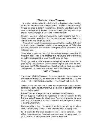
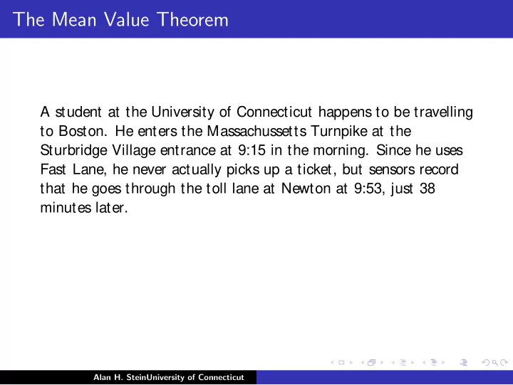
The Mean Value Theorem

A student at the University of Connecticut happens to be travelling to Boston. He enters the Massachussetts Turnpike at the Sturbridge Village entrance at 9:15 in the morning. Since he uses Fast Lane, he never actually picks up a ticket, but sensors record that he goes through the toll lane at Newton at 9:53, just 38 minutes later.

Alan H. SteinUniversity of Connecticut

The Mean Value Theorem

A student at the University of Connecticut happens to be travelling to Boston. He enters the Massachussetts Turnpike at the Sturbridge Village entrance at 9:15 in the morning. Since he uses Fast Lane, he never actually picks up a ticket, but sensors record that he goes through the toll lane at Newton at 9:53, just 38 minutes later. He soon receives a traffic summons in the mail indicating that he violated the posted speed limit and decides to appeal, since there is no indication he was caught by radar.

Alan H. SteinUniversity of Connecticut

Appearing in court, the prosecutor argues that he travelled 44.8 miles in 38 minutes and therefore travelled at an average speed of 70.74 miles per hour, more than 5 miles above the highest posted speed limit of 65 miles per hour.

Alan H. SteinUniversity of Connecticut

Appearing in court, the prosecutor argues that he travelled 44.8 miles in 38 minutes and therefore travelled at an average speed of 70.74 miles per hour, more than 5 miles above the highest posted speed limit of 65 miles per hour. The student argues that, although he may have averaged more than 65 miles per hour, there is no evidence that he actually ever travelled at an instantaneous speed of more than 65 miles per hour.

Alan H. SteinUniversity of Connecticut

Appearing in court, the prosecutor argues that he travelled 44.8 miles in 38 minutes and therefore travelled at an average speed of 70.74 miles per hour, more than 5 miles above the highest posted speed limit of 65 miles per hour. The student argues that, although he may have averaged more than 65 miles per hour, there is no evidence that he actually ever travelled at an instantaneous speed of more than 65 miles per hour. The judge considers the arguments and quickly rejects the student’s plea, noting that the Mean Value Theorem implies that since his average speed was 70.74 miles per hour, there had to be at least one instant during which his instantaneous speed was 70.74 miles per hour.

Alan H. SteinUniversity of Connecticut

Rolle’s Theorem

Alan H. SteinUniversity of Connecticut

Rolle’s Theorem

Theorem (Rolle’s Theorem)

Suppose a function f is continuous on the closed interval [a, b], differentiable on the open interval (a, b) and f (a) = f (b). Then there is a number c ∈ (a, b) such that f ′(c) = 0.

Alan H. SteinUniversity of Connecticut

Rolle’s Theorem

Theorem (Rolle’s Theorem)

Suppose a function f is continuous on the closed interval [a, b], differentiable on the open interval (a, b) and f (a) = f (b). Then there is a number c ∈ (a, b) such that f ′(c) = 0.

Geometrically, this says that if there are two points on a smooth curve takes at the same height, there must be a point in between where the tangent is horizontal.

Alan H. SteinUniversity of Connecticut

Rolle’s Theorem

Theorem (Rolle’s Theorem)

Suppose a function f is continuous on the closed interval [a, b], differentiable on the open interval (a, b) and f (a) = f (b). Then there is a number c ∈ (a, b) such that f ′(c) = 0.

Geometrically, this says that if there are two points on a smooth curve takes at the same height, there must be a point in between where the tangent is horizontal. Rolle’s Theorem is a special case of the Mean Value Theorem.

Alan H. SteinUniversity of Connecticut

Proof: Suppose f satisfies the hypotheses of Rolle’s Theorem. By

the Extreme Value Theorem for Continuous Function, there must be some point in [a, b] at which f attains a minimum and some point at which f attains a maximum.

Alan H. SteinUniversity of Connecticut

Proof: Suppose f satisfies the hypotheses of Rolle’s Theorem. By

the Extreme Value Theorem for Continuous Function, there must be some point in [a, b] at which f attains a minimum and some point at which f attains a maximum. One possibility is that f is constant on the entire interval, in which case f ′ is identically 0 on (a, b) and the conclusion is clearly true.

Alan H. SteinUniversity of Connecticut

Proof: Suppose f satisfies the hypotheses of Rolle’s Theorem. By

the Extreme Value Theorem for Continuous Function, there must be some point in [a, b] at which f attains a minimum and some point at which f attains a maximum. One possibility is that f is constant on the entire interval, in which case f ′ is identically 0 on (a, b) and the conclusion is clearly true. So let’s consider the other possibility, that f is not constant. Then either the minimum or the maximum must occur at some point

c ∈ (a, b), that is, at some point other than the endpoints.

Alan H. SteinUniversity of Connecticut

Proof: Suppose f satisfies the hypotheses of Rolle’s Theorem. By

the Extreme Value Theorem for Continuous Function, there must be some point in [a, b] at which f attains a minimum and some point at which f attains a maximum. One possibility is that f is constant on the entire interval, in which case f ′ is identically 0 on (a, b) and the conclusion is clearly true. So let’s consider the other possibility, that f is not constant. Then either the minimum or the maximum must occur at some point

c ∈ (a, b), that is, at some point other than the endpoints.

We will show that f ′(c) = 0 if f has a maximum at c. Similar reasoning would show f ′(c) = 0 if f had a minimum at c, showing the conclusion is true and completing the proof.

Alan H. SteinUniversity of Connecticut

Proof: Suppose f satisfies the hypotheses of Rolle’s Theorem. By

the Extreme Value Theorem for Continuous Function, there must be some point in [a, b] at which f attains a minimum and some point at which f attains a maximum. One possibility is that f is constant on the entire interval, in which case f ′ is identically 0 on (a, b) and the conclusion is clearly true. So let’s consider the other possibility, that f is not constant. Then either the minimum or the maximum must occur at some point

c ∈ (a, b), that is, at some point other than the endpoints.

We will show that f ′(c) = 0 if f has a maximum at c. Similar reasoning would show f ′(c) = 0 if f had a minimum at c, showing the conclusion is true and completing the proof. We know f ′(c) = limx→c

f (x) − f (c) x − c

.

Alan H. SteinUniversity of Connecticut

Proof: Suppose f satisfies the hypotheses of Rolle’s Theorem. By

the Extreme Value Theorem for Continuous Function, there must be some point in [a, b] at which f attains a minimum and some point at which f attains a maximum. One possibility is that f is constant on the entire interval, in which case f ′ is identically 0 on (a, b) and the conclusion is clearly true. So let’s consider the other possibility, that f is not constant. Then either the minimum or the maximum must occur at some point

c ∈ (a, b), that is, at some point other than the endpoints.

We will show that f ′(c) = 0 if f has a maximum at c. Similar reasoning would show f ′(c) = 0 if f had a minimum at c, showing the conclusion is true and completing the proof. We know f ′(c) = limx→c

f (x) − f (c) x − c

. Since this ordinary limit exists, it follows that both the left hand limit and the right hand limit exist and are both equal to f ′(c). We’ll consider them separately.

Alan H. SteinUniversity of Connecticut

The Left Hand Limit: f ′(c) = limx→c− f (x) − f (c) x − c

.

Alan H. SteinUniversity of Connecticut

The Left Hand Limit: f ′(c) = limx→c− f (x) − f (c) x − c

. Since f has a maximum at c, if x < c, then f (x) ≤ f (c), so

f (x) − f (c) ≤ 0. But, if x < c, it’s also true that x − c < 0 and it

follows that f (x) − f (c)

x − c ≥ 0. We see limx→c− f (x) − f (c) x − c

is the limit of non-negative numbers and therefore can’t be negative. It follows that f ′(c) ≥ 0.

Alan H. SteinUniversity of Connecticut

The Left Hand Limit: f ′(c) = limx→c− f (x) − f (c) x − c

. Since f has a maximum at c, if x < c, then f (x) ≤ f (c), so

f (x) − f (c) ≤ 0. But, if x < c, it’s also true that x − c < 0 and it

follows that f (x) − f (c)

x − c ≥ 0. We see limx→c− f (x) − f (c) x − c

is the limit of non-negative numbers and therefore can’t be negative. It follows that f ′(c) ≥ 0. The line of reasoning for the right hand limit is similar.

Alan H. SteinUniversity of Connecticut

The Right Hand Limit: f ′(c) = limx→c+ f (x) − f (c) x − c

.

Alan H. SteinUniversity of Connecticut

The Right Hand Limit: f ′(c) = limx→c+ f (x) − f (c) x − c

. Since f has a maximum at c, if x > c, then f (x) ≤ f (c), so

f (x) − f (c) ≤ 0. But, if x > c, it’s also true that x − c > 0 and it

follows that f (x) − f (c)

x − c ≤ 0. We see limx→c+ f (x) − f (c) x − c

is the limit of numbers less than or equal to 0 and therefore can’t be

• positive. It follows that f ′(c) ≤ 0.

Alan H. SteinUniversity of Connecticut

The Right Hand Limit: f ′(c) = limx→c+ f (x) − f (c) x − c

. Since f has a maximum at c, if x > c, then f (x) ≤ f (c), so

f (x) − f (c) ≤ 0. But, if x > c, it’s also true that x − c > 0 and it

follows that f (x) − f (c)

x − c ≤ 0. We see limx→c+ f (x) − f (c) x − c

is the limit of numbers less than or equal to 0 and therefore can’t be

• positive. It follows that f ′(c) ≤ 0.

Since f ′(c) ≥ 0 and f ′(c) ≤ 0, it follows that f ′(c) = 0 QED

Alan H. SteinUniversity of Connecticut

Consequences of Rolle’s Theorem

Besides being a special case of the Mean Value Theorem and being a step in the path to proving the Mean Value Theorem, Rolle’s Theorem has some interesting applications of its own.

Corollary

A polynomial equation of degree n has at most n solutions.

Alan H. SteinUniversity of Connecticut

Consequences of Rolle’s Theorem

Besides being a special case of the Mean Value Theorem and being a step in the path to proving the Mean Value Theorem, Rolle’s Theorem has some interesting applications of its own.

Corollary

Since a polynomial may be differentiated as many times as necessary, with each derivative being a polynomial of lower degree,

• ne immediate consequence of Rolle’s Theorem is that the

derivative of a polynomial has at least one zero between each pair

• f distinct zeros of the original polynomial.

Alan H. SteinUniversity of Connecticut

Since a polynomial may be differentiated as many times as necessary, with each derivative being a polynomial of lower degree,

• ne immediate consequence of Rolle’s Theorem is that the

derivative of a polynomial has at least one zero between each pair

• f distinct zeros of the original polynomial.

The derivative of a linear polynomial is a non-zero constant, having no zeros, so a linear polynomial can’t have more than 1 zero.

Alan H. SteinUniversity of Connecticut

Since a polynomial may be differentiated as many times as necessary, with each derivative being a polynomial of lower degree,

• ne immediate consequence of Rolle’s Theorem is that the

derivative of a polynomial has at least one zero between each pair

• f distinct zeros of the original polynomial.

The derivative of a linear polynomial is a non-zero constant, having no zeros, so a linear polynomial can’t have more than 1 zero. The derivative of a quadratic polynomial is linear, having no more than 1 zero, so a quadratic can’t have more than 2 zeros.

Alan H. SteinUniversity of Connecticut

Since a polynomial may be differentiated as many times as necessary, with each derivative being a polynomial of lower degree,

• ne immediate consequence of Rolle’s Theorem is that the

derivative of a polynomial has at least one zero between each pair

• f distinct zeros of the original polynomial.

The derivative of a linear polynomial is a non-zero constant, having no zeros, so a linear polynomial can’t have more than 1 zero. The derivative of a quadratic polynomial is linear, having no more than 1 zero, so a quadratic can’t have more than 2 zeros. The derivative of a cubic polynomial is quadratic, having no more than 2 zeros, so the cubic can’t have more than 3 zeros.

Alan H. SteinUniversity of Connecticut

Since a polynomial may be differentiated as many times as necessary, with each derivative being a polynomial of lower degree,

• ne immediate consequence of Rolle’s Theorem is that the

derivative of a polynomial has at least one zero between each pair

• f distinct zeros of the original polynomial.

The derivative of a linear polynomial is a non-zero constant, having no zeros, so a linear polynomial can’t have more than 1 zero. The derivative of a quadratic polynomial is linear, having no more than 1 zero, so a quadratic can’t have more than 2 zeros. The derivative of a cubic polynomial is quadratic, having no more than 2 zeros, so the cubic can’t have more than 3 zeros. This clearly goes on forever. The argument can be made rigorous through the use of Mathematical Induction.

Alan H. SteinUniversity of Connecticut

The Mean Value Theorem

Alan H. SteinUniversity of Connecticut

The Mean Value Theorem

Theorem (The Mean Value Theorem)

Suppose a function f is continuous on the closed interval [a, b] and differentiable on the open interval (a, b). Then there is a number c ∈ (a, b) such that f (b) − f (a) = f ′(c)(b − a) or, equivalently, f ′(c) = f (b) − f (a) b − a .

Alan H. SteinUniversity of Connecticut

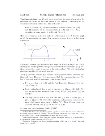
The Mean Value Theorem

Theorem (The Mean Value Theorem)

Suppose a function f is continuous on the closed interval [a, b] and differentiable on the open interval (a, b). Then there is a number c ∈ (a, b) such that f (b) − f (a) = f ′(c)(b − a) or, equivalently, f ′(c) = f (b) − f (a) b − a .

Geometrically, the Mean Value Theorem says that if there is a smooth curve connecting two points, there must be some point in between at which the tangent line is parallel to the line connecting those two points.

Alan H. SteinUniversity of Connecticut

The Mean Value Theorem

Theorem (The Mean Value Theorem)

Suppose a function f is continuous on the closed interval [a, b] and differentiable on the open interval (a, b). Then there is a number c ∈ (a, b) such that f (b) − f (a) = f ′(c)(b − a) or, equivalently, f ′(c) = f (b) − f (a) b − a .

Geometrically, the Mean Value Theorem says that if there is a smooth curve connecting two points, there must be some point in between at which the tangent line is parallel to the line connecting those two points. Analytically, the Mean Value Theorem says the rate of change of a differentiable function must, at some point, take on its average, or

mean value.

Alan H. SteinUniversity of Connecticut

The proof of the Mean Value Theorem depends on the fact that the particular point at which the tangent line is parallel to the line connecting the endpoints also happens to be the point at which the curve is furthers away from that line. The proof essentially consists of applying Rolle’s Theorem to the function measuring the distance between the line and the curve.

Alan H. SteinUniversity of Connecticut

Since the line goes between the points (a, f (a)) and (b, f (b)), its slope will be f (b) − f (a)

b − a

and its equation may be written, in point-slope form,

Alan H. SteinUniversity of Connecticut

Since the line goes between the points (a, f (a)) and (b, f (b)), its slope will be f (b) − f (a)

b − a

and its equation may be written, in point-slope form,

y − f (a) = f (b) − f (a) b − a · (x − a).

Alan H. SteinUniversity of Connecticut

Since the line goes between the points (a, f (a)) and (b, f (b)), its slope will be f (b) − f (a)

b − a

and its equation may be written, in point-slope form,

y − f (a) = f (b) − f (a) b − a · (x − a).

Solving for y, we may write the equation in the form

Alan H. SteinUniversity of Connecticut

Since the line goes between the points (a, f (a)) and (b, f (b)), its slope will be f (b) − f (a)

b − a

and its equation may be written, in point-slope form,

y − f (a) = f (b) − f (a) b − a · (x − a).

Solving for y, we may write the equation in the form

y = f (a) + f (b) − f (a) b − a · (x − a).

Alan H. SteinUniversity of Connecticut

Since the line goes between the points (a, f (a)) and (b, f (b)), its slope will be f (b) − f (a)

b − a

and its equation may be written, in point-slope form,

y − f (a) = f (b) − f (a) b − a · (x − a).

Solving for y, we may write the equation in the form

y = f (a) + f (b) − f (a) b − a · (x − a).

Since the second coordinate of a point on the curve with first coordinate x is f (x), the vertical distance between the line and the curve will equal

Alan H. SteinUniversity of Connecticut

Since the line goes between the points (a, f (a)) and (b, f (b)), its slope will be f (b) − f (a)

b − a

and its equation may be written, in point-slope form,

y − f (a) = f (b) − f (a) b − a · (x − a).

Solving for y, we may write the equation in the form

y = f (a) + f (b) − f (a) b − a · (x − a).

Since the second coordinate of a point on the curve with first coordinate x is f (x), the vertical distance between the line and the curve will equal

f (x) −

• f (a) + f (b) − f (a)

b − a · (x − a)

• =

Alan H. SteinUniversity of Connecticut

Since the line goes between the points (a, f (a)) and (b, f (b)), its slope will be f (b) − f (a)

b − a

and its equation may be written, in point-slope form,

y − f (a) = f (b) − f (a) b − a · (x − a).

Solving for y, we may write the equation in the form

y = f (a) + f (b) − f (a) b − a · (x − a).

Since the second coordinate of a point on the curve with first coordinate x is f (x), the vertical distance between the line and the curve will equal

f (x) −

• f (a) + f (b) − f (a)

b − a · (x − a)

• =

f (x) − f (a) − f (b) − f (a) b − a · (x − a).

Alan H. SteinUniversity of Connecticut

Since the line goes between the points (a, f (a)) and (b, f (b)), its slope will be f (b) − f (a)

b − a

and its equation may be written, in point-slope form,

y − f (a) = f (b) − f (a) b − a · (x − a).

Solving for y, we may write the equation in the form

y = f (a) + f (b) − f (a) b − a · (x − a).

Since the second coordinate of a point on the curve with first coordinate x is f (x), the vertical distance between the line and the curve will equal

f (x) −

• f (a) + f (b) − f (a)

b − a · (x − a)

• =

f (x) − f (a) − f (b) − f (a) b − a · (x − a).

We are now prepared to prove the Mean Value Theorem.

Alan H. SteinUniversity of Connecticut

Proof: Let φ(x) = f (x) − f (a) − f (b) − f (a) b − a · (x − a).

Alan H. SteinUniversity of Connecticut

Proof: Let φ(x) = f (x) − f (a) − f (b) − f (a) b − a · (x − a).

It is easy to see that φ satisfies the hypotheses of Rolle’s Theorem

• n the interval [a, b]. Certainly, the fact that φ is both continuous

and differentiable on [a, b] follows immediately from the fact that f

• is. In addition,

Alan H. SteinUniversity of Connecticut

Proof: Let φ(x) = f (x) − f (a) − f (b) − f (a) b − a · (x − a).

It is easy to see that φ satisfies the hypotheses of Rolle’s Theorem

• n the interval [a, b]. Certainly, the fact that φ is both continuous

and differentiable on [a, b] follows immediately from the fact that f

• is. In addition,

φ(a) = f (a) − f (a) − f (b) − f (a) b − a · (a − a) = 0

Alan H. SteinUniversity of Connecticut

Proof: Let φ(x) = f (x) − f (a) − f (b) − f (a) b − a · (x − a).

It is easy to see that φ satisfies the hypotheses of Rolle’s Theorem

• n the interval [a, b]. Certainly, the fact that φ is both continuous

and differentiable on [a, b] follows immediately from the fact that f

• is. In addition,

φ(a) = f (a) − f (a) − f (b) − f (a) b − a · (a − a) = 0

and

Alan H. SteinUniversity of Connecticut

Proof: Let φ(x) = f (x) − f (a) − f (b) − f (a) b − a · (x − a).

It is easy to see that φ satisfies the hypotheses of Rolle’s Theorem

• n the interval [a, b]. Certainly, the fact that φ is both continuous

and differentiable on [a, b] follows immediately from the fact that f

• is. In addition,

φ(a) = f (a) − f (a) − f (b) − f (a) b − a · (a − a) = 0

and

φ(b) = f (b) − f (a) − f (b) − f (a) b − a · (b − a) = f (b) − f (a) − [f (b) − f (a)] = 0.

Alan H. SteinUniversity of Connecticut

Proof: Let φ(x) = f (x) − f (a) − f (b) − f (a) b − a · (x − a).

It is easy to see that φ satisfies the hypotheses of Rolle’s Theorem

• n the interval [a, b]. Certainly, the fact that φ is both continuous

and differentiable on [a, b] follows immediately from the fact that f

• is. In addition,

φ(a) = f (a) − f (a) − f (b) − f (a) b − a · (a − a) = 0

and

φ(b) = f (b) − f (a) − f (b) − f (a) b − a · (b − a) = f (b) − f (a) − [f (b) − f (a)] = 0.

Thus, there must be some c ∈ (a, b) such that φ′(c) = 0. We first

• btain φ′(c) as follows.

Alan H. SteinUniversity of Connecticut

φ′(x) = f ′(x) − f (b) − f (a) b − a

Alan H. SteinUniversity of Connecticut

φ′(x) = f ′(x) − f (b) − f (a) b − a φ′(c) = f ′(c) − f (b) − f (a) b − a

Alan H. SteinUniversity of Connecticut

φ′(x) = f ′(x) − f (b) − f (a) b − a φ′(c) = f ′(c) − f (b) − f (a) b − a

Since φ′(c) = 0, it follows that

Alan H. SteinUniversity of Connecticut

φ′(x) = f ′(x) − f (b) − f (a) b − a φ′(c) = f ′(c) − f (b) − f (a) b − a

Since φ′(c) = 0, it follows that

f ′(c) − f (b) − f (a) b − a

= 0.

Alan H. SteinUniversity of Connecticut

φ′(x) = f ′(x) − f (b) − f (a) b − a φ′(c) = f ′(c) − f (b) − f (a) b − a

Since φ′(c) = 0, it follows that

f ′(c) − f (b) − f (a) b − a

= 0.

f ′(c) = f (b) − f (a) b − a

Alan H. SteinUniversity of Connecticut

φ′(x) = f ′(x) − f (b) − f (a) b − a φ′(c) = f ′(c) − f (b) − f (a) b − a

Since φ′(c) = 0, it follows that

f ′(c) − f (b) − f (a) b − a

= 0.

f ′(c) = f (b) − f (a) b − a f ′(c)(b − a) = f (b) − f (a)

QED

Alan H. SteinUniversity of Connecticut

Consequences of the Mean Value Theorem

Perhaps the most important consequence of the Mean Value

Theorem is that it gives precise meaning to the most important

single concept in elementary Calculus,

Alan H. SteinUniversity of Connecticut

The Derivative Measures Rate of Change.

Theorem

• a. If the derivative of a function is positive at all points on an

interval, then the function is increasing on that interval.

• b. If the derivative of a function is negative at all points on an

interval, then the function is decreasing on that interval.

Alan H. SteinUniversity of Connecticut

To prove this, we need a precise definition of what it means to be increasing or decreasing.

Alan H. SteinUniversity of Connecticut

To prove this, we need a precise definition of what it means to be increasing or decreasing.

Definition (Strictly Increasing)

A function f is said to be strictly increasing on an open interval I if f (a) < f (b) whenever a, b ∈ I and a < b.

Alan H. SteinUniversity of Connecticut

To prove this, we need a precise definition of what it means to be increasing or decreasing.

Definition (Strictly Increasing)

A function f is said to be strictly increasing on an open interval I if f (a) < f (b) whenever a, b ∈ I and a < b.

Definition (Nondecreasing)

A function f is said to be nondecreasing on an open interval I if

f (a) ≤ f (b) whenever a, b ∈ I and a < b.

Alan H. SteinUniversity of Connecticut

To prove this, we need a precise definition of what it means to be increasing or decreasing.

Definition (Strictly Increasing)

A function f is said to be strictly increasing on an open interval I if f (a) < f (b) whenever a, b ∈ I and a < b.

Definition (Nondecreasing)

A function f is said to be nondecreasing on an open interval I if

f (a) ≤ f (b) whenever a, b ∈ I and a < b.

Note the subtle difference. Often, we will simply say a function is

• increasing. Generally, in those cases, it will not really be important

whether we mean strictly increasing or simply nondecreasing.

Alan H. SteinUniversity of Connecticut

To prove this, we need a precise definition of what it means to be increasing or decreasing.

Definition (Strictly Increasing)

A function f is said to be strictly increasing on an open interval I if f (a) < f (b) whenever a, b ∈ I and a < b.

Definition (Nondecreasing)

A function f is said to be nondecreasing on an open interval I if

f (a) ≤ f (b) whenever a, b ∈ I and a < b.

Note the subtle difference. Often, we will simply say a function is

• increasing. Generally, in those cases, it will not really be important

whether we mean strictly increasing or simply nondecreasing. There are similar definitions of the terms strictly decreasing and

• nonincreasing. Here, too, we will often use the ambiguous term

decreasing.

Alan H. SteinUniversity of Connecticut

Definition (Strictly Decreasing)

A function f is said to be strictly decreasing on an open interval I if f (a) > f (b) whenever a, b ∈ I and a < b.

Alan H. SteinUniversity of Connecticut

Definition (Strictly Decreasing)

A function f is said to be strictly decreasing on an open interval I if f (a) > f (b) whenever a, b ∈ I and a < b.

Definition (Nonincreasing)

A function f is said to be nonincreasing on an open interval I if

f (a) ≥ f (b) whenever a, b ∈ I and a < b.

Alan H. SteinUniversity of Connecticut

Definition (Strictly Decreasing)

A function f is said to be strictly decreasing on an open interval I if f (a) > f (b) whenever a, b ∈ I and a < b.

Definition (Nonincreasing)

A function f is said to be nonincreasing on an open interval I if

f (a) ≥ f (b) whenever a, b ∈ I and a < b.

With these definitions, we are ready to prove the derivative

measures rate of change. We will prove just one of what are really

four different parts, that if the derivative is strictly positive then the function is strictly increasing.

Alan H. SteinUniversity of Connecticut

Proof.

Suppose f ′(x) > 0

∀x ∈ I and let a, b ∈ I, a < b. We need to

prove that f (a) < f (b).

Alan H. SteinUniversity of Connecticut

Proof.

Suppose f ′(x) > 0

∀x ∈ I and let a, b ∈ I, a < b. We need to

prove that f (a) < f (b).

Note: We’ve introduced the notation ∀ to mean for all or for every.

Alan H. SteinUniversity of Connecticut

Proof.

Suppose f ′(x) > 0

∀x ∈ I and let a, b ∈ I, a < b. We need to

prove that f (a) < f (b).

Note: We’ve introduced the notation ∀ to mean for all or for every.

Since f ′(x) > 0

∀x ∈ I, it follows that f is continuous on [a, b]

and differentiable on (a, b), so by the Mean Value Theorem there is some c ∈ (a, b) such that f (b) − f (a) = f ′(c)(b − a).

Alan H. SteinUniversity of Connecticut

Proof.

Suppose f ′(x) > 0

∀x ∈ I and let a, b ∈ I, a < b. We need to

prove that f (a) < f (b).

Note: We’ve introduced the notation ∀ to mean for all or for every.

Since f ′(x) > 0

∀x ∈ I, it follows that f is continuous on [a, b]

and differentiable on (a, b), so by the Mean Value Theorem there is some c ∈ (a, b) such that f (b) − f (a) = f ′(c)(b − a). Since f ′(x) > 0

∀x ∈ I, it follows that f ′(c) is positive. Since a < b, it follows that b − a is also positive, so that f ′(c)(b − a) is

also positive and hence f (b) − f (a) must be positive.

Alan H. SteinUniversity of Connecticut

Proof.

Suppose f ′(x) > 0

∀x ∈ I and let a, b ∈ I, a < b. We need to

prove that f (a) < f (b).

Note: We’ve introduced the notation ∀ to mean for all or for every.

Since f ′(x) > 0

∀x ∈ I, it follows that f is continuous on [a, b]

and differentiable on (a, b), so by the Mean Value Theorem there is some c ∈ (a, b) such that f (b) − f (a) = f ′(c)(b − a). Since f ′(x) > 0

∀x ∈ I, it follows that f ′(c) is positive. Since a < b, it follows that b − a is also positive, so that f ′(c)(b − a) is

also positive and hence f (b) − f (a) must be positive. Clearly, f (a) must be smaller than f (b).

Alan H. SteinUniversity of Connecticut

Very Different Functions Can’t Have the Same Derivative

Alan H. SteinUniversity of Connecticut

Very Different Functions Can’t Have the Same Derivative

It’s obvious that if two functions differ by only a constant term, then they will have the same derivative.

Alan H. SteinUniversity of Connecticut

Very Different Functions Can’t Have the Same Derivative

It’s obvious that if two functions differ by only a constant term, then they will have the same derivative. Example: d

dx

• x2

= d

dx

• x2 + 5
• = 2x.

Alan H. SteinUniversity of Connecticut

Very Different Functions Can’t Have the Same Derivative

It’s obvious that if two functions differ by only a constant term, then they will have the same derivative. Example: d

dx

• x2

= d

dx

• x2 + 5
• = 2x.

A natural question is whether only functions differing by a constant can share the same derivative. The Mean Value Theorem enables us to see this is true.

Alan H. SteinUniversity of Connecticut

Theorem

If f ′(x) = g′(x) for all x in some interval, then there is some constant k such that f (x) = g(x) + k.

Alan H. SteinUniversity of Connecticut

Theorem

If f ′(x) = g′(x) for all x in some interval, then there is some constant k such that f (x) = g(x) + k. Proof: Let φ = f − g and let a be some fixed point in the interval.

Now let x be in the interval. Clearly, the φ is both continuous and differentiable on the interval with endpoints a and x and we can apply the Mean Value Theorem.

Alan H. SteinUniversity of Connecticut

Theorem

If f ′(x) = g′(x) for all x in some interval, then there is some constant k such that f (x) = g(x) + k. Proof: Let φ = f − g and let a be some fixed point in the interval.

Now let x be in the interval. Clearly, the φ is both continuous and differentiable on the interval with endpoints a and x and we can apply the Mean Value Theorem.

We use that language because it is possible that a < x and the interval is [a, x] but also possible that a > x and the interval is

[x, a].

Alan H. SteinUniversity of Connecticut

By the Mean Value Theorem, there is some c in the interval such that φ(x) − φ(a) = φ′(c)(x − a).

Alan H. SteinUniversity of Connecticut

By the Mean Value Theorem, there is some c in the interval such that φ(x) − φ(a) = φ′(c)(x − a). Because φ = f − g, it follows that φ′(c) = 0, so φ(x) − φ(a) = 0.

Alan H. SteinUniversity of Connecticut

By the Mean Value Theorem, there is some c in the interval such that φ(x) − φ(a) = φ′(c)(x − a). Because φ = f − g, it follows that φ′(c) = 0, so φ(x) − φ(a) = 0. It follows that φ(x) = φ(a), or φ(x) = k, where we let k = φ(a).

Alan H. SteinUniversity of Connecticut

By the Mean Value Theorem, there is some c in the interval such that φ(x) − φ(a) = φ′(c)(x − a). Because φ = f − g, it follows that φ′(c) = 0, so φ(x) − φ(a) = 0. It follows that φ(x) = φ(a), or φ(x) = k, where we let k = φ(a). Since φ = f − g, we have f (x) − g(x) = k, or f (x) = g(x) + k. QED

Alan H. SteinUniversity of Connecticut

Corollary

Only constant functions have derivatives which are identically 0.

Alan H. SteinUniversity of Connecticut

Corollary

Only constant functions have derivatives which are identically 0.

This theorem will prove useful when we try to find functions with a given derivative. One application will be to determine the acceleration due to gravity.

Alan H. SteinUniversity of Connecticut

Example

An object is dropped from a height of 128 feet. How long does it take to reach the ground?

Alan H. SteinUniversity of Connecticut

Example

An object is dropped from a height of 128 feet. How long does it take to reach the ground?

Solution

Alan H. SteinUniversity of Connecticut

Example

An object is dropped from a height of 128 feet. How long does it take to reach the ground?

Solution

Let:

◮ h be the height of the object, measured in feet. ◮ v be the velocity of the object, measured in feet per second. ◮ t be the time since the object was dropped, measured in

seconds.

Alan H. SteinUniversity of Connecticut

We Know:

◮ h = 128 when t = 0 ◮ v = 0 when t = 0 ◮ dh

dt = v (Since velocity is the rate at which the height

changes.)

◮ dv

dt = −32 (Since acceleration is the rate at which the velocity

changes and the acceleration due to gravity is 32 feet per second per second and is in the downward, or negative, direction.)

Alan H. SteinUniversity of Connecticut

frame

◮ The value of t when h = 0

Alan H. SteinUniversity of Connecticut

Since d

dt (−32t) = −32 and two functions can have the same

derivative only if they differ by a constant, it follows that

Alan H. SteinUniversity of Connecticut

Since d

dt (−32t) = −32 and two functions can have the same

derivative only if they differ by a constant, it follows that

v = −32t + c for some constant c.

Alan H. SteinUniversity of Connecticut

Since d

dt (−32t) = −32 and two functions can have the same

derivative only if they differ by a constant, it follows that

v = −32t + c for some constant c.

Since v = 0 when t = 0, it follows that

Alan H. SteinUniversity of Connecticut

Since d

dt (−32t) = −32 and two functions can have the same

derivative only if they differ by a constant, it follows that

v = −32t + c for some constant c.

Since v = 0 when t = 0, it follows that 0 = −32 · 0 + c

Alan H. SteinUniversity of Connecticut

Since d

dt (−32t) = −32 and two functions can have the same

derivative only if they differ by a constant, it follows that

v = −32t + c for some constant c.

Since v = 0 when t = 0, it follows that 0 = −32 · 0 + c

c = 0

Alan H. SteinUniversity of Connecticut

Since d

dt (−32t) = −32 and two functions can have the same

derivative only if they differ by a constant, it follows that

v = −32t + c for some constant c.

Since v = 0 when t = 0, it follows that 0 = −32 · 0 + c

c = 0 v = −32t

Alan H. SteinUniversity of Connecticut

Since d

dt

• −16t2

= −32t, dh

dt = v = −32t and two functions can

have the same derivative only if they differ by a constant, it follows that

Alan H. SteinUniversity of Connecticut

Since d

dt

• −16t2

= −32t, dh

dt = v = −32t and two functions can

have the same derivative only if they differ by a constant, it follows that

h = −16t2 + k for some constant k.

Alan H. SteinUniversity of Connecticut

Since d

dt

• −16t2

= −32t, dh

dt = v = −32t and two functions can

have the same derivative only if they differ by a constant, it follows that

h = −16t2 + k for some constant k.

Since h = 128 when t = 0, it follows that

Alan H. SteinUniversity of Connecticut

Since d

dt

• −16t2

= −32t, dh

dt = v = −32t and two functions can

have the same derivative only if they differ by a constant, it follows that

h = −16t2 + k for some constant k.

Since h = 128 when t = 0, it follows that 128 = −16 · 02 + k

Alan H. SteinUniversity of Connecticut

Since d

dt

• −16t2

= −32t, dh

dt = v = −32t and two functions can

have the same derivative only if they differ by a constant, it follows that

h = −16t2 + k for some constant k.

Since h = 128 when t = 0, it follows that 128 = −16 · 02 + k

k = 128

Alan H. SteinUniversity of Connecticut

Since d

dt

• −16t2

= −32t, dh

dt = v = −32t and two functions can

have the same derivative only if they differ by a constant, it follows that

h = −16t2 + k for some constant k.

Since h = 128 when t = 0, it follows that 128 = −16 · 02 + k

k = 128 h = −16t2 + 128

Alan H. SteinUniversity of Connecticut

Thus, when h = 0,

Alan H. SteinUniversity of Connecticut

Thus, when h = 0, 0 = −16t2 + 128

Alan H. SteinUniversity of Connecticut

Thus, when h = 0, 0 = −16t2 + 128 16t2 = 128

Alan H. SteinUniversity of Connecticut

Thus, when h = 0, 0 = −16t2 + 128 16t2 = 128

t2 = 128

16 = 8

Alan H. SteinUniversity of Connecticut

Thus, when h = 0, 0 = −16t2 + 128 16t2 = 128

t2 = 128

16 = 8

t = √

8 = 2

√

2 ≈ 2.828

Alan H. SteinUniversity of Connecticut

Thus, when h = 0, 0 = −16t2 + 128 16t2 = 128

t2 = 128

16 = 8

t = √

8 = 2

√

2 ≈ 2.828 It thus takes 2

√

2 seconds for the object to fall to the ground.

Alan H. SteinUniversity of Connecticut

Thus, when h = 0, 0 = −16t2 + 128 16t2 = 128

t2 = 128

16 = 8

t = √

8 = 2

√

2 ≈ 2.828 It thus takes 2

√

2 seconds for the object to fall to the ground.

We can also figure out how fast it was going when it hit the ground:

Alan H. SteinUniversity of Connecticut

Thus, when h = 0, 0 = −16t2 + 128 16t2 = 128

t2 = 128

16 = 8

t = √

8 = 2

√

2 ≈ 2.828 It thus takes 2

√

2 seconds for the object to fall to the ground.

We can also figure out how fast it was going when it hit the ground:

Since v = −32t, when t = 2

√

2 we have

v = −32 · 2 √

2 = −64

√

2 ≈ −90.510, so the object is travelling at a speed of 64

√

2 feet per second when it hits the ground.

Alan H. SteinUniversity of Connecticut

Example

Determine the acceleration due to gravity.

Alan H. SteinUniversity of Connecticut

Example

Determine the acceleration due to gravity.

Solution:

Alan H. SteinUniversity of Connecticut

Example

Determine the acceleration due to gravity.

Solution:

We may perform the following experiment: We drop a coin from the ceiling and measure the time it takes to hit the ground.

Alan H. SteinUniversity of Connecticut

Let:

Alan H. SteinUniversity of Connecticut

Let:

◮ t be the time since the coin is dropped ◮ T be the amount of time it takes to hit the ground ◮ h be the height of the coin ◮ H be the height of the ceiling ◮ v be the speed of the coin ◮ g be the acceleration due to gravity

Alan H. SteinUniversity of Connecticut

We Know

We know:

Alan H. SteinUniversity of Connecticut

We Know

We know:

◮ dh

dt = v

◮ dv

dt = g

◮ h = H when t = 0 ◮ v = 0 when t = 0 ◮ h = 0 when t = T

Alan H. SteinUniversity of Connecticut

We Want

We want:

Alan H. SteinUniversity of Connecticut

We Want

We want:

◮ The value of g.

Alan H. SteinUniversity of Connecticut

Since d

dt (gt) = g, dv dt = g and two functions can have the same

derivative only if they differ by a constant, it follows that

Alan H. SteinUniversity of Connecticut

Since d

dt (gt) = g, dv dt = g and two functions can have the same

derivative only if they differ by a constant, it follows that

v = gt + c for some constant c.

Alan H. SteinUniversity of Connecticut

Since d

dt (gt) = g, dv dt = g and two functions can have the same

derivative only if they differ by a constant, it follows that

v = gt + c for some constant c.

Since v = 0 when t = 0, it follows that

Alan H. SteinUniversity of Connecticut

Since d

dt (gt) = g, dv dt = g and two functions can have the same

derivative only if they differ by a constant, it follows that

v = gt + c for some constant c.

Since v = 0 when t = 0, it follows that 0 = g · 0 + c

Alan H. SteinUniversity of Connecticut

Since d

dt (gt) = g, dv dt = g and two functions can have the same

derivative only if they differ by a constant, it follows that

v = gt + c for some constant c.

Since v = 0 when t = 0, it follows that 0 = g · 0 + c

c = 0

Alan H. SteinUniversity of Connecticut

Since d

dt (gt) = g, dv dt = g and two functions can have the same

derivative only if they differ by a constant, it follows that

v = gt + c for some constant c.

Since v = 0 when t = 0, it follows that 0 = g · 0 + c

c = 0 v = gt

Alan H. SteinUniversity of Connecticut

Since d

dt 1

2gt2

= gt, dh

dt = v = gt and two functions can have

the same derivative only if they differ by a constant, it follows that

Alan H. SteinUniversity of Connecticut

Since d

dt 1

2gt2

= gt, dh

dt = v = gt and two functions can have

the same derivative only if they differ by a constant, it follows that

h =

1 2gt2 + k for some constant k.

Alan H. SteinUniversity of Connecticut

Since d

dt 1

2gt2

= gt, dh

dt = v = gt and two functions can have

the same derivative only if they differ by a constant, it follows that

h =

1 2gt2 + k for some constant k.

Since h = H when t = 0, it follows that

Alan H. SteinUniversity of Connecticut

Since d

dt 1

2gt2

= gt, dh

dt = v = gt and two functions can have

the same derivative only if they differ by a constant, it follows that

h =

1 2gt2 + k for some constant k.

Since h = H when t = 0, it follows that

H =

1 2g · 02 + k

Alan H. SteinUniversity of Connecticut

Since d

dt 1

2gt2

= gt, dh

dt = v = gt and two functions can have

the same derivative only if they differ by a constant, it follows that

h =

1 2gt2 + k for some constant k.

Since h = H when t = 0, it follows that

H =

1 2g · 02 + k

k = H

Alan H. SteinUniversity of Connecticut

Since d

dt 1

2gt2

= gt, dh

dt = v = gt and two functions can have

the same derivative only if they differ by a constant, it follows that

h =

1 2gt2 + k for some constant k.

Since h = H when t = 0, it follows that

H =

1 2g · 02 + k

k = H h =

1 2gt2 + H

Alan H. SteinUniversity of Connecticut

Since h = 0 when t = T, it follows that

Alan H. SteinUniversity of Connecticut

Since h = 0 when t = T, it follows that 0 =

1 2gT 2 + H

Alan H. SteinUniversity of Connecticut

Since h = 0 when t = T, it follows that 0 =

1 2gT 2 + H 1 2gT 2 = −H

Alan H. SteinUniversity of Connecticut

Since h = 0 when t = T, it follows that 0 =

1 2gT 2 + H 1 2gT 2 = −H

g = −H

1 2T 2

Alan H. SteinUniversity of Connecticut

Since h = 0 when t = T, it follows that 0 =

1 2gT 2 + H 1 2gT 2 = −H

g = −H

1 2T 2

g = −2H T 2

Alan H. SteinUniversity of Connecticut

Since h = 0 when t = T, it follows that 0 =

1 2gT 2 + H 1 2gT 2 = −H

g = −H

1 2T 2

g = −2H T 2

So the acceleration due to gravity is 2H

T 2 feet per second per

• second. Note that g is negative, since the acceleration is

downward.

Alan H. SteinUniversity of Connecticut