The IPCC process: results and further questions Natural climate - PowerPoint PPT Presentation
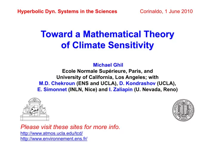
Hyperbolic Dyn. Systems in the Sciences Corinaldo, 1 June 2010 Michael Ghil Ecole Normale Suprieure, Paris, and University of California, Los Angeles; with M.D. Chekroun (ENS and UCLA), D. Kondrashov (UCLA), E. Simonnet (INLN, Nice) and I.
Hyperbolic Dyn. Systems in the Sciences Corinaldo, 1 June 2010 Michael Ghil Ecole Normale Supérieure, Paris, and University of California, Los Angeles; with M.D. Chekroun (ENS and UCLA), D. Kondrashov (UCLA), E. Simonnet (INLN, Nice) and I. Zaliapin (U. Nevada, Reno) Please visit these sites for more info. http://www.atmos.ucla.edu/tcd/ http://www.environnement.ens.fr/
• The IPCC process: results and further questions � • Natural climate variability as a source of uncertainties � – sensitivity to initial data error growth � – sensitivity to model formulation see below! � • Uncertainties and how to fix them � – structural in/stability � – random dynamical systems (RDS) � • Two or more illustrative examples � – Arnol ʼ d tongues and a ʻʻ French garden ʼʼ� – the Lorenz system � – an ENSO “toy” model � • Linear response theory and climate sensitivity � • Conclusions, work in progress and references �
Unfortunately, things Unfortunately, things aren ’ ’ t t all all that easy! that easy! aren What to do? Try to achieve better interpretation of, and agreement between, models … Ghil, M ., 2002: Natural climate variability, in Encyclopedia of Global Environmental Change , T. Munn (Ed.), Vol. 1, Wiley
Temperatures rise: • What about impacts? • How to adapt? The answer, my friend, is blowing in the wind, i.e ., it depends on the accuracy and reliability of the forecast … Source : IPCC (2007), AR4, WGI, SPM
It’s gotta do with us, at least a bit, ain’t it? But just how much? IPCC (2007)
• The IPCC process: results and further questions � • Natural climate variability as a source of uncertainties � – sensitivity to initial data error growth � – sensitivity to model formulation see below! � • Uncertainties and how to fix them � – structural in/stability � – random dynamical systems (RDS) � • Two or more illustrative examples � – Arnol ʼ d tongues and a ʻʻ French garden ʼʼ� – the Lorenz system � – an ENSO “toy” model � • Linear response theory and climate sensitivity � • Conclusions, work in progress and references �
Courtesy Tim Palmer, 2009 �
• The IPCC process: results and further questions. � • Natural climate variability as a source of uncertainties � – sensitivity to initial data error growth � – sensitivity to model formulation see below! � • Uncertainties and how to fix them � – structural in/stability � – random dynamical systems (RDS) � • Two or more illustrative examples � – Arnol ʼ d tongues and a ʻʻ French garden ʼʼ� – the Lorenz system � – an ENSO “toy” model � • Linear response theory and climate sensitivity � • Conclusions, work in progress and references �
The uncertainties might be intrinsic , rather than mere “tuning problems” If so, maybe stochastic structural stability could help! Might fit in nicely with recent taste for “stochastic parameterizations” The DDS dream of structural stability (from Abraham & Marsden , 1978)
So what’ ’s it s it gonna gonna be like, by 2100? be like, by 2100? So what
Non-autonomous Dynamical Systems A linear example as a paradigm Let us first start with a very difficult problem: ˙ Study the “dynamics" of x = − α x + σ t , α, σ > 0 . (1) First remarks: The system ˙ x = − α x , i.e. the autonomous part of (1), is dissipative. All the solutions of ˙ x = − α x , converge towards 0 as t → + ∞ . Is it the case for (1)? Certainly not! The autonomous part is forced; we even introduce an infinite energy ❘ + ∞ over an infinite horizon: t d t = + ∞ ! 0 Forward attraction seems to be ill adapted to time-dependent forcing. Goal: Find a concept of attraction such that: (i) It is compatible with the forward concept, when there is no forcing, (ii) It provides a way to assess the effect of dissipation in some sense. For that let’s do some computations... Michael Ghil Toward a Mathematical Theory of Climate Sensitivity
Non-autonomous Dynamical Systems A linear example as a paradigm Let us first start with a very difficult problem: ˙ Study the “dynamics" of x = − α x + σ t , α, σ > 0 . (1) First remarks: The system ˙ x = − α x , i.e. the autonomous part of (1), is dissipative. All the solutions of ˙ x = − α x , converge towards 0 as t → + ∞ . Is it the case for (1)? Certainly not! The autonomous part is forced; we even introduce an infinite energy ❘ + ∞ over an infinite horizon: t d t = + ∞ ! 0 Forward attraction seems to be ill adapted to time-dependent forcing. Goal: Find a concept of attraction such that: (i) It is compatible with the forward concept, when there is no forcing, (ii) It provides a way to assess the effect of dissipation in some sense. For that let’s do some computations... Michael Ghil Toward a Mathematical Theory of Climate Sensitivity
Non-autonomous Dynamical Systems A linear example as a paradigm Let us first start with a very difficult problem: ˙ Study the “dynamics" of x = − α x + σ t , α, σ > 0 . (1) First remarks: The system ˙ x = − α x , i.e. the autonomous part of (1), is dissipative. All the solutions of ˙ x = − α x , converge towards 0 as t → + ∞ . Is it the case for (1)? Certainly not! The autonomous part is forced; we even introduce an infinite energy ❘ + ∞ over an infinite horizon: t d t = + ∞ ! 0 Forward attraction seems to be ill adapted to time-dependent forcing. Goal: Find a concept of attraction such that: (i) It is compatible with the forward concept, when there is no forcing, (ii) It provides a way to assess the effect of dissipation in some sense. For that let’s do some computations... Michael Ghil Toward a Mathematical Theory of Climate Sensitivity
Non-autonomous Dynamical Systems Commentaries We’ve just shown that: | x ( t , s ; x 0 ) − a ( t ) | − s →−∞ 0 ; for every t fixed , → all initial data x 0 , with a ( t ) = σ α ( t − 1 /α ) . We’ve just encountered the concept of pullback attraction; here { a ( t ) } is the pullback attractor of the system (1). What does it means physically? The pullback attractor provides a way to assess an asymptotic regime at time t — the time at which we observe the system — for a system starting to evolve from the remote past s , s << t . Thus, this asymptotic regime evolves with time: it is a dynamical object. The effect of dissipation is now viewed via this dynamical object and not a static one, as a strange attractor does for autonomous systems. Michael Ghil Toward a Mathematical Theory of Climate Sensitivity
Non-autonomous Dynamical Systems Commentaries We’ve just shown that: | x ( t , s ; x 0 ) − a ( t ) | − s →−∞ 0 ; for every t fixed , → all initial data x 0 , with a ( t ) = σ α ( t − 1 /α ) . We’ve just encountered the concept of pullback attraction; here { a ( t ) } is the pullback attractor of the system (1). What does it means physically? The pullback attractor provides a way to assess an asymptotic regime at time t — the time at which we observe the system — for a system starting to evolve from the remote past s , s << t . Thus, this asymptotic regime evolves with time: it is a dynamical object. The effect of dissipation is now viewed via this dynamical object and not a static one, as a strange attractor does for autonomous systems. Michael Ghil Toward a Mathematical Theory of Climate Sensitivity
Random Dynamical Systems - RDS theory This theory is a combination of measure (probability) theory and dynamical systems developed by the “Bremen group" (L.Arnold, 1998). It allows one to treat Stochastic Differential Equations ( SDEs ), and more general systems driven by some “noise," as flows . Setting: (i) A phase space X . Example : R n . (ii) A probability space (Ω , F , P ) . Example : The Wiener space Ω = C 0 ( R ; R n ) with Wiener measure P = γ . (iii) A model of the noise θ ( t ) : Ω → Ω that preserves the measure P , i.e. θ ( t ) P = P ; θ is called the driving system. Example : W ( t , θ ( s ) ω ) = W ( t + s , ω ) − W ( s , ω ) ; it starts the noise at s instead of t = 0. (iv) A mapping ϕ : R × Ω × X → X with the cocycle property. Example : The solution of an SDE. Michael Ghil Toward a Mathematical Theory of Climate Sensitivity
Random Dynamical Systems - A geometric view of SDEs ϕ is a random dynamical system (RDS) Θ( t )( x , ω ) = ( θ ( t ) ω, ϕ ( t , ω ) x ) is a flow on the bundle Michael Ghil Toward a Mathematical Theory of Climate Sensitivity
Random Dynamical Systems - Random attractor A random attractor A ( ω ) is both invariant and “pullback" attracting : (a) Invariant : ϕ ( t , ω ) A ( ω ) = A ( θ ( t ) ω ) . (b) Attracting : ∀ B ⊂ X , lim t →∞ dist ( ϕ ( t , θ ( − t ) ω ) B , A ( ω )) = 0 a.s. Michael Ghil Toward a Mathematical Theory of Climate Sensitivity
Recommend
More recommend
Explore More Topics
Stay informed with curated content and fresh updates.
