The intersection axiom of conditional independence : some new - PowerPoint PPT Presentation

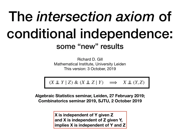
The intersection axiom of conditional independence : some “new” results Richard D. Gill Mathematical Institute, University Leiden This version: 3 October, 2019 ( X ⊥ ⊥ Y ∣ Z ) & ( X ⊥ ⊥ Z ∣ Y ) ⟹ X ⊥ ⊥ ( Y , Z ) Algebraic Statistics seminar, Leiden, 27 February 2019; Combinatorics seminar 2019, SJTU, 2 October 2019 X is independent of Y given Z and X is independent of Z given Y, implies X is independent of Y and Z

The intersection axiom of conditional independence : some “new” results Intersection axiom. Well known to be neither Richard D. Gill true nor even an axiom. Mathematical Institute, University Leiden This version: 2 October, 2019 ( X ⊥ ⊥ Y ∣ Z ) & ( X ⊥ ⊥ Z ∣ Y ) ⟹ X ⊥ ⊥ ( Y , Z ) Algebraic Statistics seminar, Leiden, 27 February 2019; Combinatorics seminar 2019, JTSU, 2 October 2019 X is independent of Y given Z and X is independent of Z given Y, implies X is independent of Y and Z

Comfort zones All variables have: • Finite outcome space [Nice for algebraic geometry] • Countable outcome space • Continuous joint density with respect to sigma-finite product measures [Usually not used rigorously] • Outcome spaces are Polish ❤ Other “convenience” assumptions: Strictly positive joint density Multivariate normal also allows algebraic geometry approach

Inspiration: study group Algebraic Statistics on algebraic statistics Seth Sullivant North Carolina State University E-mail address : smsulli2@ncsu.edu 2010 Mathematics Subject Classification. Primary 62-01, 14-01, 13P10, 13P15, 14M12, 14M25, 14P10, 14T05, 52B20, 60J10, 62F03, 62H17, 90C10, 92D15 Key words and phrases. algebraic statistics, graphical models, contingency tables, conditional independence, phylogenetic models, design of experiments, Gr¨ obner bases, real algebraic geometry, exponential families, exact test, maximum likelihood degree, Markov basis, disclosure limitation, random graph models, model selection, identifiability Abstract. Algebraic statistics uses tools from algebraic geometry, com- mutative algebra, combinatorics, and their computational sides to ad- dress problems in statistics and its applications. The starting point for this connection is the observation that many statistical models are semialgebraic sets. The algebra/statistics connection is now over twenty Graduate Studies in Mathematics years old– this book presents the first comprehensive and introductory Volume: 194; 2018; 490 pp; Hardcover treatment of the subject. After background material in probability, al- MSC: Primary 62; 14; 13; 52; 60; 90; 92; gebra, and statistics, the book covers a range of topics in algebraic statistics including algebraic exponential families, likelihood inference, Print ISBN: 978-1-4704-3517-2 Fisher’s exact test, bounds on entries of contingency tables, design of experiments, identifiability of hidden variable models, phylogenetic mod- els, and model selection. The book is suitable for both classroom use and independent study, as it has numerous examples, references, and over 150 exercises.

The (semi-)graphoid axioms of (conditional) independence 1. Symmetry X ⊥ ⊥ Y ⟹ Y ⊥ ⊥ X 2. Decomposition X ⊥ ⊥ ( Y , Z ) ⟹ X ⊥ ⊥ Y 3. Weak union X ⊥ ⊥ ( Y , Z ) ⟹ X ⊥ ⊥ Y ∣ Z ( X ⊥ ⊥ Z ∣ Y & X ⊥ ⊥ Y ) 4. Contraction ⟹ X ⊥ ⊥ ( Y , Z ) 5. Intersection ( X ⊥ ⊥ Y ∣ Z & X ⊥ ⊥ Z ∣ Y ) ⟹ X ⊥ ⊥ ( Y , Z ) 1–5: (with further global conditioning): the graphoid axioms. Phil Dawid (1980). 1–4: ( … ): the semi-graphoid axioms So called because of similarity to *graph separation* for subgraphs of a simple undirected graph: A is separated from B by C

• The intersection axiom (nr 5): ( X ⊥ ⊥ Y ∣ Z ) & ( X ⊥ ⊥ Z ∣ Y ) ⟹ X ⊥ ⊥ ( Y , Z ) • “New” result: ( X ⊥ ⊥ Y ∣ Z ) & ( X ⊥ ⊥ Z ∣ Y ) ⟺ X ⊥ ⊥ ( Y , Z ) ∣ W where W:= f(Y) = g(Z) for some f, g • In particular, we can take W = Law((Y, Z) | X) • If f and g are trivial (constant) we obtain “axiom 5” • Also “new”: Nontrivial f, g exist such that f(Y) = g(Z) a.e. i ff A, B exist with probabilities strictly between 0 and 1 s.t. Pr( Y ∈ A & Z ∈ B c ) = 0 = Pr( Y ∈ A c & Z ∈ B ) Call such a joint law decomposable

• The intersection axiom: ( X ⊥ ⊥ Y ∣ Z ) & ( X ⊥ ⊥ Z ∣ Y ) ⟹ X ⊥ ⊥ ( Y , Z ) • “New” result: ( X ⊥ ⊥ Y ∣ Z ) & ( X ⊥ ⊥ Z ∣ Y ) ⟺ X ⊥ ⊥ ( Y , Z ) ∣ W where W:= f(Y) = g(Z) for some f, g • In particular, we can take W = Law((Y, Z) | X) • If f and g are trivial (constant) we obtain “axiom 5” • Also “new”: Nontrivial f, g exist such that f(Y) = g(Z) a.e. i ff A, B exist with probabilities strictly between 0 and 1 s.t. Pr( Y ∈ A & Z ∈ B c ) = 0 = Pr( Y ∈ A c & Z ∈ B ) Call such a joint law decomposable

• The intersection axiom: ( X ⊥ ⊥ Y ∣ Z ) & ( X ⊥ ⊥ Z ∣ Y ) ⟹ X ⊥ ⊥ ( Y , Z ) • “New” result: ( X ⊥ ⊥ Y ∣ Z ) & ( X ⊥ ⊥ Z ∣ Y ) ⟺ X ⊥ ⊥ ( Y , Z ) ∣ W where W:= f(Y) = g(Z) for some f, g • In particular, we can take W = Law((Y, Z) | X) • If f and g are trivial (constant) we obtain “axiom 5” • Also “new”: Nontrivial f, g exist such that f(Y) = g(Z) a.e. i ff A, B exist with probabilities strictly between 0 and 1 s.t. Pr( Y ∈ A & Z ∈ B c ) = 0 = Pr( Y ∈ A c & Z ∈ B ) Call such a joint law decomposable

• The intersection axiom: ( X ⊥ ⊥ Y ∣ Z ) & ( X ⊥ ⊥ Z ∣ Y ) ⟹ X ⊥ ⊥ ( Y , Z ) • “New” result: ( X ⊥ ⊥ Y ∣ Z ) & ( X ⊥ ⊥ Z ∣ Y ) ⟺ X ⊥ ⊥ ( Y , Z ) ∣ W where W:= f(Y) = g(Z) for some f, g • In particular, we can take W = Law((Y, Z) | X) • If f and g are trivial (constant) we obtain “axiom 5” • Also “new”: Nontrivial f, g exist such that f(Y) = g(Z) a.e. i ff A, B exist with probabilities strictly between 0 and 1 s.t. Pr( Y ∈ A & Z ∈ B c ) = 0 = Pr( Y ∈ A c & Z ∈ B ) Call such a joint law decomposable

Construction of counter example

More elaborate counter example Leading to the general theorem

Proof of new rule Discrete case

Comfort zones • All variables have finite support (Algebraic Geometry) • All variables have countable support • All variables have continuous joint probability densities (many applied statisticians) • All densities are strictly positive • All distributions are non-degenerate Gaussian • All variables take values in Polish spaces (My favourite) Polish space: a topological space which can be given a metric making it complete and separable

Please recall • The joint probability distribution of X and Y can be disintegrated into the marginal distribution of X and a family of conditional distribution s of Y given X = x • The disintegration is unique up to almost everywhere equivalence • Conditional independence of X and Y given Z is just ordinary independence within each of the joint laws of X and Y conditional on Z = z • For me, 0/0 = “undefined” and 0 x “undefined” = 0 (probability times number) • So: conditional distributions do exist if we condition on zero probability events; they’re just not uniquely defined. • The non-uniqueness is harmless

Some new notation • I’ll denote by “law( X )” the probability distribution (law) of X , where X is a random variable which takes values in a space 𝒴 . So law( X ) is a probability distribution on 𝒴 • In the finite, discrete case, a “law” is just a vector of real numbers, non-negative, adding to one. • In the Polish case, the set of probability laws on a given Polish space is itself a Polish space under, e.g., the Wasserstein metric. Disintegrations exist, Everything is nice. • The family of conditional distributions of X given Y, (law( X | Y = y )) y ∈ 𝒵 can be thought of as a function of y ∈ 𝒵 . In the Polish case, the function is Borel measurable. • As a function of the random variable Y , we can consider it as a random variable, or as a random vector talking values in an a ffi ne space. • By Law( X | Y ) I’ll denote that random variable, taking values in the space of probability laws on 𝒴 . Note distinction: Law vs. law

Crucial lemma X ⫫ Y | Law( X | Y )

Lemma: X ⫫ Y | Law( X | Y ) 𝝚 d = probability simplex, dimension d capital L = Law(X | Y), a random probability measure Small 𝓂 (“ell”) is a possible realisation Proof of lemma, discrete case Recall, X ⫫ Y | Z ⟺ p(x, y, z) = g(x, z) h(y, z) Thus X ⫫ Y | L ⟺ we can factor p(x, y, l) this way Given function p(x, y), pick any x ∈ 𝒴 , y ∈ 𝒵 , ℓ ∈ Δ | 𝒴 | − 1 p ( x , y , ℓ ) = p ( x , y ) ⋅ 1{ ℓ = p ( ⋅ , y )/ p ( y )} = ℓ ( x ) p ( y )1{ ℓ = p ( ⋅ , y )/ p ( y )} = Eval ( ℓ , x ) . p ( y )1{ ℓ = p ( ⋅ , y )/ p ( y )} Proof of lemma, Polish case Similar, but a tiny bit di ff erent – we don’t assume existence of joint densities!

Proof of forwards implication • X ⫫ Y | Z ⟹ Law( X | Y, Z ) = Law( X | Z ) • X ⫫ Z | Y ⟹ Law( X | Y, Z ) = Law( X | Y ) • So we have w(Y, Z) = g(Z) = f(Y) = : W for some functions w, g, f • By our lemma, X ⫫ ( Y, Z ) | Law( X | ( Y, Z )) • We found functions g, f such that g(Z) = f(Y) and, with W:= w(Y, Z) = g(Z) = f(Y) , X ⫫ ( Y, Z ) | W

Proof of reverse implication • Suppose X ⫫ ( Y, Z ) | W where W = g(Z) = f(Y) for some functions g, f • By axiom 3, X ⫫ Y | ( W, Z ) • So X ⫫ Y | ( g(Z), Z ) • So X ⫫ Y | Z • Similarly, X ⫫ Z | Y