The IITM Earth System Model: Development and Future Road Map Swapna - - PowerPoint PPT Presentation

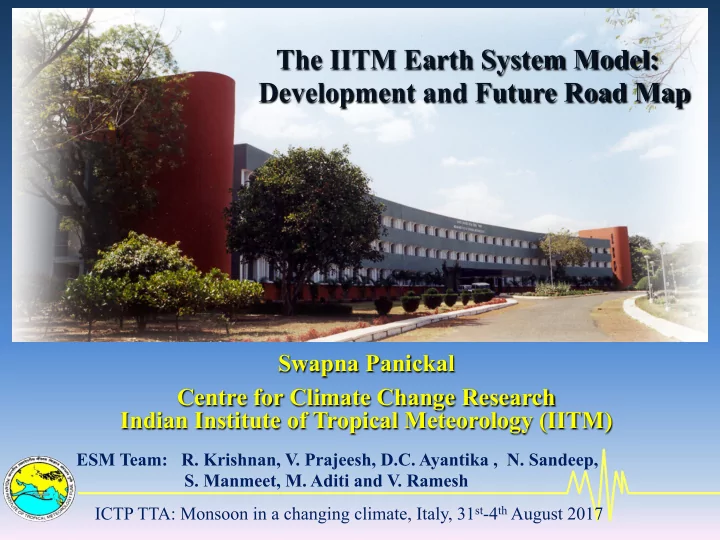
The IITM Earth System Model: Development and Future Road Map

ESM Team: R. Krishnan, V. Prajeesh, D.C. Ayantika , N. Sandeep,

• S. Manmeet, M. Aditi and V. Ramesh

Swapna Panickal Centre for Climate Change Research Indian Institute of Tropical Meteorology (IITM)

ICTP TTA: Monsoon in a changing climate, Italy, 31st-4th August 2017

• Climate Modeling : brief history
• Need for Improving Monsoon Simulation
• Overview of IITM-ESM
• Step towards Earth System Modeling frame-work
• Future Road Map

Outline

ICTP TTA: Monsoon in a changing climate, Italy, 31st-4th August 2017

Manabe and Brian (1969)

• Recognized as a “milestone in

scientific computing”, Nature (2006).

• Sector model of 120o
• 1 atmospheric year coupled to
• 100 ocean years
• 1200h for 1 simulated year
• (0.02 SYPD) on Univac 1108

Ø Empirical evidence indicates that poleward heat transport by ocean currents is of same order of magnitude as poleward transport

• f energy in the atmosphere (Sverdrup, 1975)

Ø Serious attempt to calculate climate must take into account atmosphere and hydrosphere Climate Calculations with a Combined Ocean-Atmosphere Model

Atmospheric response to doubled CO2

Manabe and Wetherald (1975): A foundational document of climate modeling

• Estimated the temperature changes resulting from doubling CO2 concentration
• Simplified three-dimensional general circulation model.
• A limited computational domain, an idealized topography, no beat transport

by ocean currents, and fixed cloudiness.

• The CO2 increase raises the temperature of the model troposphere and

significantly increases the intensity of the hydrologic cycle

The Charney Report (1979)

“Carbon dioxide and climate: A Scientific Assessment.”

• Precursor to the IPCC Assessment Reports.
• Based on 5 model runs: 3 from Manabe (GFDL), 2 from Hansen

(GISS).

• Conclusions:
• Direct radiative effects due to doubling of CO2: 4 W/m2
• Feedbacks: water vapor (Clausius-Clapeyron), snow-ice albedo

feedback.

• Cloud effects: “How important the cloud effects are, is, however, an

extremely difficult question to answer. The cloud distribution is a property of the entire climate system, in which many other feedbacks are involved.”

• “We believe, therefore, that the equilibrium surface warming will be

in the range of 1.5-4.5C, with the most probable value near 3C.”

Climate Modeling Today...

IPCC AR5. 20th century warming cannot be explained without greenhouse gas forcings IPCC AR5 SPM:

• Warming of the climate system is

unequivocal

• Last three decades has been

successively warmer than any preceding decade since 1850

IPCC, 2013

Recent Climate Change Report

Planet has warmed by 0.85 K over 1880-2012

Climate Change 2013: WG1 contribution to IPCC Fifth Assessment Report

Wide varia)ons among CMIP5/ CMIP3 models in capturing the South Asian monsoon

Realism of present-day climate simula4on is an essen4al requirement for reliable assessment of future changes in monsoon

Source: Kripalani et al. 2010 CMIP3 vs Obs Source: Sharmila Sur et al. 2014 ISM domain 15S-30N, 50E-120E Indian Land: CMIP5 vs Obs

Trend in All India Summer Monsoon Rainfall

Historical and SRES A1B projection of South Asian monsoon rainfall [Turner and Annamalai, 2012]

• Observed data shows a negative trend in precipitation since 1950.
• Decadal variability dominates & considerable uncertainty in precipitation

between the models

Temporal evolution of monsoon hydro-climatic signals

Krishnan et al. 2016

• Decreasing trend of monsoon precipitation during the later part of 20th century
• The aridity index (SPEI , Standard Precipitation-Evaporation Index] indicates

a marked increase in propensity of monsoon droughts

Guhathakurtha and Rajeevan, 2006: Trends in monsoon rainfall over India (1901-2003) Significant negative trends: Kerala, Jharkhand, Chattisgarh

Long-term trends in the Indian monsoon rainfall

The 142-yr (1871-2012) record of all-India monsoon rainfall indicates a 40% increase in the frequency of monsoon-droughts during the second half relative to the first half of the period

Summer Monsoon Rainfall and Crop Production

Detrended All India Kharif Production Anomaly (NCC, IMD)

• 2
• 2
• 1
• 1
• 5

0. 5. 10 15 20 25

• 25.00
• 20.00
• 15.00
• 10.00
• 5.00

0.00 5.00 10.00 15.00 20.00 25.00 1966 1969 1972 1975 1978 1981 1984 1987 1990 1993 1996 1999 2002 2005

ANOMALY Vs ISMR

Crop Production ISMR

Rainfall - 2009

Impact of a severe drought on GDP remains 2 to 5% throughout, despite the substantial decrease in the contribution of agriculture to GDP over the five decades. Two-thirds of the workforce is in agriculture Gadgil and Gadgil (2006)

GDP and Indian Monsoon Rainfall

(Chung and Ramanathan 2006)

The observed linear trend shows widespread decrease in rainfall over the IGP and mountainous west-coast. The increasing trend over southeastern China and adjoining areas is also observed. The prominent drought over the Sahel region is also evident from the decreasing trend.

Observed Trend in Summer Rainfall 1950 to 2002

Ø Most models show an intensified Asian monsoon rainfall, Ø There is substantial model spread. (Li and Ting, 2016) The linear trend of area averaged land precipitation from 2006 to 2099 for India and eastern China from CMIP5 Models

Ø In a warmer climate, as a consequence of the increase in tropospheric water vapor, the global hydrological cycle will become more intensified (Held and Soden 2006). Ø The rate of precipitation increase is less than the rate of water vapor, and tropical atmospheric circulation weakens as climate warms (Vecchi and Soden 2007, Krishnan et al., 2015) Ø The atmospheric circulation is the major source of uncertainty in regional rainfall projection (Xie et al. 2015) Why there are uncertainty in regional precipitation response ?

• Start with an atmosphere-ocean coupled model with

realistic mean climate

– Fidelity in capturing the global and monsoon climate – Realistic representation of monsoon interannual variability – Features of ocean-atmosphere coupled interactions – …

• Include components / modules of the ESM

– Biogeochemistry – Interactive Sea-ice – Aerosol and Chemistry Transport – …

Roadmap for Earth System Model (ESM) development

Science of climate change

Detection, attribution & projection of global climate and regional monsoons

Atmosphere: T126 spectral (~ 190 km), 64 ver)cal levels – ESMv1 Ocean : 0.5 deg grid, ~ 0.25 deg between 10N-10S, 40 ver)cal levels

• The NCEP CFS Components
• Atmospheric GFS (Global Forecast System) model

– T62 ; vertical: 64 sigma – pressure hybrid levels – Model top 0.2 mb – Revised Simplified Arakawa-Schubert convection (Han & Pan) – Non-local PBL (Pan & Hong) – SW radiation (Chou, modifications by Y. Hou) – Prognostic cloud water (Moorthi, Hou & Zhao) – LW radiation (GFDL, AER in operational wx model) – Land surface processes (Noah land model)

• Interactive Ocean: GFDL MOM4p1 (Modular Ocean Model-4p1)

– 1.0 deg poleward of 10oN and 10oS; and 0.33 deg near equator (10oS – 10oN) – 50 levels – Interactive sea-ice – Interactive ocean biogeochemistry

IITM Earth System Model (IITM ESM) Based on Coupled Forecast System (CFS) T62L64

GFS (Atmospheric Model) with NOAH Land Model AO Coupler

fast loop slow loop

GFDL MOM4p1 (Ocean Model) & SIS (Ice Model) Atm Grid Sea Ice Ocean

FMS coupler

Global mean surface (2m) temperature Annual mean SST difference (Model minus WOA)

ESM CFSv2

CFSv2 ESM1.0

Tropical SST

The drift in surface temperature and SST is minimum in IITM ESMv1 (red line) compared to CFSv2 (blue line). Significant reduction in cold SST bias in tropical IO and subtropical Pacific

Differences between simulated and observed long-term global-mean

• cean temperature as a function of depth and time.

GFDL CM2.0 GFDL CM2.1 ESM1.0 CFSv2 Coupled models drift towards a more equilibrated state. Initial rapid cooling of SST followed by warming trend. Significant subsurface drifts seen through multiple centuries

• f simulation. Vertical redistribution of heat with tendency of cooling in upper layers and

warming in the sub-surface – Delworth et al. 2006

Precipitation (mm day-1): JJAS mean CFSv2 ESM1.0 TRMM

Inter-annual variability

PDO - IITM ESM

HadISST ESMv1 CFSV2 CFSV2 ESMv1 HadISST

Nino3 SST

‏

Precipitation (5N-35N; 65E-95E)‏

Precipitation‏

Seasonal cycle of precipitation and Nino 3 SST is captured in ESM & CFSv2

Lagged correlation between ISMR and Nino3 SST in the preceding/following months are captured well in IITM ESM as compared to CFSv2

ENSO-Monsoon relationship PDO-Monsoon relationship

Recent improvements in IITM ESM

Boreal summer monsoon (JJAS) precipitation and bias

Depletion of NH sea-ice during Jan-Mar

Obs ESMv1

Weakening of AMOC

Sea-Ice concentration & AMOC

Black line is the preindustrial run. The red line shows the 20th century simulation and the 21st century portion of the SRES A1B simulation (stared from the end of the 20th century simulation. The blue line shows the 22nd and 23rd century SRES A1B simulation

Time-series of TOA energy budget (GFDL2.1 CM9) – V. Lucarini, F. Ragone, 2011, Rev. Geophy

NDSW – Net downward Short wave radiation OLW- Outgoing Long wave radiation DLW- Downward Long wave (depends on T of Atm) ULW – Upward long wave (depends on T of Ocean) SHF – Sensible heat flux LHF – Latent heat flux Surface Flux = NDSW – DLW +ULW +SHF+LHF

Net flux = TOA – Surface flux

Courtesy: Prajeesh

Energy Balance of the Coupled System

NDSW – Net downward Short wave flux at TOA OLW – Outgoing Longwave flux (depends on layer temperature according to Stefan Boltzman law) NDSW

Internal Energy (CpT) Kinetic Energy (Winds)

• Incr. Temp

(Friction) Minimize atmospheric energy loss – Bretherton et al. 2012

TOA Energy Balance

Energy Balance in IITM ESM

Preindustrial TOA (Wm-2) Energy imbalance for CMIP5 Models (Forster et al., 2013)

Net Radia)on (W m-2) at TOA

IITM-ESMv2 Obs (CERES)

Energy Balance in IITM ESM

Net flux TOA (W m-2) Net Flux Surface (W m-2) Difference (W m-2) ESMv1 (T126) 6.6 1.2 5.4 ESMv2 (T62) 0.80 0.81 0.01

Sea-Ice concentration and AMOC in IITM ESMv2

Data Courtesy : Bjorn Stevens, Stefan Kinne (Max Planck) Prescribed )me-varying aerosol distribu)ons in IITM ESM from CMIP Aerosol forcing in IITM ESM AF (TOA) AF (Surface)

Aerosol TOA forcing (total sky)= -0.9 Courtesy: Ayan)ka, CCCR

Land use/land cover changes (Hurtt et al., 2015) Pre industrial (1850) Present day (2007)

Courtesy: Sandeep, CCCR

• f

Klima (German for ‘climate’)

41

“DECK”: Development

CMIP DECK

Evaluation Characterisation CMIP6 Concept: A Distributed Organization under the oversight of the CMIP Panel

CMIP6 Schematic

CMIP6 experimental design

Meehl et al., 2014: Climate Model Intercomparisons: Preparing for the Next Phase, Eos Trans. AGU, 95,77-84.

Experiment C M I P 6 label Experiment Description F o r c i n g methods Start Year End Year Minimum # Years Major purpose Historical AMIP amip Observed SSTs and SICs prescribed CO2 concentration- driven 1979 2014 36 Evaluation Pre-industrial control piControl Coupled atmosphere/ocean pre- industrial control run (concentration driven) CO2 emission-

• r

concentration- driven 1850 n/a 500 Evaluation, unforced variability 1 %/yr CO2 1pctCO2 CO2 prescribed to increase at 1%/yr until concentrations have quadrupled, and then (optionally) extended 160 years with CO2 concentration held constant CO2 concentration- driven n/a n/a 140 Climate sensitivity, feedbacks Quadruple CO2 abruptly, then hold fixed abrupt4xCO 2 CO2 abruptly quadrupled and then held constant CO2 concentration- driven n/a n/a 150 Climate sensitivity, feedbacks, fast responses Past ~1.5 centuries historical Simulation of the recent past CO2 emission-

• r

concentration- driven 1850 2014 165 Evaluation

CMIP6 Experiments

• Significant reduction of cold bias of global mean SST by ~0.8oC
• ENSO & PDO are robust and spatially more coherent in IITM ESM
• ENSO and monsoon links are well-captured
• The IITM Earth System Model: Transformation of a Seasonal

Prediction Model to a Long Term Climate Model. Swapna et al. (BAMS, 2015). Ø Reduced the TOA energy imbalance Ø Improved the mean precipitation over Asian region Ø Improved the sea ice distribution Ø Included time-varying aerosol concentration Ø Corrected the hydrology imbalance Ø Improved representation of ocean BGC

IITM ESMv1 IITM ESMv2

Summary

• Development of High Resolution Global Model (~grid size 27 km)

Atmospheric version of IITM-ESM for dynamical downscaling. Generation of high resolution global climate and monsoon projections.

• High-resolution IITM-ESM coupled model (atmosphere grid size: 27

km, ocean grid: 0.5 deg x 0.5 deg and 0.25 deg x 0.25 deg near equator) for long-term climate.

• Development of next-generation IITM-ESM coupled model, to include

new components (eg., interactive aerosols, chemistry, carbon cycle).

Future Roadmap