The Himalaya of Bhutan Intro to Quantitative Geology - PowerPoint PPT Presentation
Introduction to Quantitative Geology Overview of Exercises 6 and 7 Quantitative t hermochronology Instructor: David Whipp david.whipp@helsinki.fi 2.12.19 Intro to Quantitative Geology www.helsinki.fi/yliopisto 1 The Himalaya of Bhutan Intro
Introduction to Quantitative Geology Overview of Exercises 6 and 7 Quantitative t hermochronology Instructor: David Whipp david.whipp@helsinki.fi 2.12.19 Intro to Quantitative Geology www.helsinki.fi/yliopisto 1
The Himalaya of Bhutan Intro to Quantitative Geology www.helsinki.fi/yliopisto 2 http://commons.wikimedia.org
Thermochronometer ages in western Bhutan Coutand et al., 2014 Intro to Quantitative Geology www.helsinki.fi/yliopisto 3
Linking ages to geological processes a) 14 Western Transect 9 13 (89.1-89.82°E) 12 I-STD 8 MCT 11 7 10 MBT Elevation (± 1 σ ) Elevation asl (km) Age (Ma) 9 MFT 6 8 5 7 6 4 5 3 4 3 2 2 1 1 0 0 Coutand et al., 2014 Latitude (°N) 28.25 28.5 26.5 26.75 27 27.25 27.5 27.75 28 0 50 100 150 200 Distance along swath (km) • b) Thermochronometer ages contain valuable information about past geological processes, but age interpretation is difficult Intro to Quantitative Geology www.helsinki.fi/yliopisto 4 )
Estimating rock exhumation rates Grand Teton National Park, Wyoming, USA • In mountainous settings, rock exhumation is the result of a erosional (surface) and/or tectonic processes • Exhumation : The unroofing history of a rock, as caused by tectonic and/or surficial processes (Ring et al., 1999) Intro to Quantitative Geology www.helsinki.fi/yliopisto 5
Estimating exhumation rates from ages • The simplest way to estimate a long-term average exhumation rate from a thermochronometer age is to assume a constant geothermal gradient and determine the depth from which the sample was exhumed • For example, assume we measure an apatite (U-Th)/He age of 12.3±0.9 Ma in a sample • Assume a nominal closure temperature 𝑈 c of 75±5°C and a “typical” geothermal gradient of 20°C/km • How would you find the exhumation rate? • The simple approach is to find the depth of 𝑈 c and divide that depth by the age Intro to Quantitative Geology www.helsinki.fi/yliopisto 6
Estimating exhumation rates from ages • The simplest way to estimate a long-term average exhumation rate from a thermochronometer age is to assume a constant geothermal gradient and determine the depth from which the sample was exhumed • For example, assume we measure an apatite (U-Th)/He age of 12.3±0.9 Ma in a sample • Assume a nominal closure temperature 𝑈 c of 75±5°C and a “typical” geothermal gradient of 20°C/km • How would you find the exhumation rate? • The simple approach is to find the depth of 𝑈 c and divide that depth by the age Intro to Quantitative Geology www.helsinki.fi/yliopisto 7
Exhumation rate example • If we assume the surface temperature is 0°C, the depth 𝑨 c of 𝑈 c is simply 𝑈 c divided by the geothermal gradient • 𝑨 c = 75°C / (20°C/km) = 3.75 km • An exhumation rate ė can be estimated by dividing that depth by the measured age • ė = 3.75 km / 12.3 Ma = ~0.3 km/Ma = ~0.3 mm/a Intro to Quantitative Geology www.helsinki.fi/yliopisto 8
A constant thermal gradient is a bad idea • This approach works, but it neglects many known thermal factors including ‘bending’ of the geotherm as a result of thermal advection • A more reasonable approach would be to utilize a 1-D thermal model to simulate heat transfer processes during rock cooling, which will be our approach in the final two lab exercises Intro to Quantitative Geology www.helsinki.fi/yliopisto 9
1-D steady-state geotherms • Advection is often the main thermal influence on thermochronometer ages in mountainous regions • Thus, advection must be considered by using an appropriate equation ✓ 1 − e − ( v z z/ κ ) ◆ T ( z ) = T L 1 − e − ( v z L/ κ ) Intro to Quantitative Geology www.helsinki.fi/yliopisto 10
Now what? • With a predicted 1-D thermal field, the next step is to determine the cooling history for a rock sample • We know the sample is at the surface ( 𝑨 = 0) today, and we can use the advection velocity 𝑤 𝑨 to determine the cooling history • How? • We can calculate the past depth of a rock sample by using time steps back to some time in the past • Each time step, the rock will be displaced by 𝑤 𝑨 ⨉ 𝑒𝑢 Intro to Quantitative Geology www.helsinki.fi/yliopisto 11
Now what? • With a predicted 1-D thermal field, the next step is to determine the cooling history for a rock sample • We know the sample is at the surface ( 𝑨 = 0) today, and we can use the advection velocity 𝑤 𝑨 to determine the cooling history • How? • We can calculate the past depth of a rock sample by using time steps back to some time in the past • Each time step, the rock will be displaced by 𝑤 𝑨 ⨉ 𝑒𝑢 Intro to Quantitative Geology www.helsinki.fi/yliopisto 12
Generating a thermal history • At each time, record the depth and temperature, 𝑈 5 ( 𝑨 , 𝑢 ) then move the particle 𝑈 4 ( 𝑨 , 𝑢 ) upward by 𝑤 𝑨 ⨉ 𝑒𝑢 Predicted age 𝑈 3 ( 𝑨 , 𝑢 ) 𝑈 2 ( 𝑨 , 𝑢 ) • 𝑈 1 ( 𝑨 , 𝑢 ) The result is a thermal 𝑈 c history for a given exhumation (advection) rate that can now be linked to an estimated closure temperature to predict a cooling age and compare to data Intro to Quantitative Geology www.helsinki.fi/yliopisto 13
General concept for age prediction Predicted ages Measured age Age 1. Calculate thermal solution 2. Generate thermal history based on thermal solution and advection velocity 3. Use thermal history to calculate 𝑈 c 4. Record time at which sample cools below 𝑈 c (predicted age) 5. Compare predicted age to measured age 6. Repeat steps 1-5 as needed until a good fit is observed Intro to Quantitative Geology www.helsinki.fi/yliopisto 14
Recommend
More recommend
Explore More Topics
Stay informed with curated content and fresh updates.
