The Frequency Domain Time domain methods: regress present on past; - PowerPoint PPT Presentation

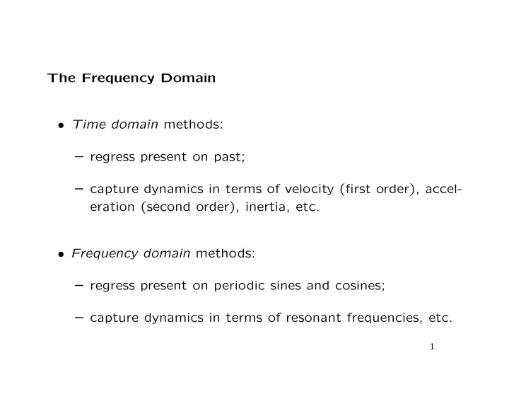
The Frequency Domain • Time domain methods: – regress present on past; – capture dynamics in terms of velocity (first order), accel- eration (second order), inertia, etc. • Frequency domain methods: – regress present on periodic sines and cosines; – capture dynamics in terms of resonant frequencies, etc. 1

E.g. AR(2): plot(ts(arima.sim(list(order = c(2,0,0), ar = c(1.5,-.95)), n = 144))) • Strong periodicity, around 16 peaks ⇒ period of around 9 samples. • Fitting an AR model doesn’t describe this: x t = 1 . 50 x t − 1 − 0 . 95 x t − 2 + w t . 2

Cyclical Behavior • Simplest case is the periodic process x t = A cos(2 πωt + φ ) = U 1 cos(2 πωt ) + U 2 sin(2 πωt ) . where: – A is amplitude ; – ω is frequency , in cycles per sample; – φ is phase , in radians; • and U 1 = A cos( φ ), U 2 = − A sin( φ ). 3

Folding Frequency; Aliasing • If ω = 0, x t = A cos( φ ), constant. • If ω = 1? At t = 0 , 1 , 2 , . . . , same thing! • ω = 0 is an alias of ω = 1. • All frequencies higher than ω = 1 / 2 have an alias in 0 ≤ ω ≤ 1 / 2: cos[2 π ( k ± ω ) t + φ ] = cos(2 πωt ± φ ) , t = 0 , 1 , 2 , . . . • ω = 1 / 2 is the folding frequency . 4

• For example, ω = 0 . 8: omega = 0.8; phi = pi / 6; plot(function(x) cos(2 * pi * omega * x + phi), from = 0, to = 10); plot(function(x) cos(2 * pi * (1 - omega) * x - phi), from = 0, to = 10, add = TRUE, col = "red"); abline(v = 0:10, lty = 2, col = "blue"); • Note: – ω = 0 . 8 = 0 . 5 + 0 . 3, and 1 − ω = 0 . 2 = 0 . 5 − 0 . 3; – 1 − ω is ω “folded” around 0 . 5. 5

Stationarity • If x t = A cos(2 πωt + φ ) = U 1 cos(2 πωt ) + U 2 sin(2 πωt ) . and φ is random, uniformly distributed on [0 , 2 π ), then: E( x t ) = 0 , = 1 2 A 2 cos(2 πωh ) . � � E x t + h x t • So x t is weakly stationary. 6

• Also E( U 1 ) = E( U 2 ) = 0 , = 1 U 2 U 2 2 A 2 , � � � � E = E 1 2 and E( U 1 U 2 ) = 0 . • Alternatively, if the U ’s have these properties, x t is stationary with the same mean and autocovariances: E( x t ) = 0 , = 1 2 A 2 cos(2 πωh ) . � � E x t + h x t 7

• More generally, if q � � � x t = U k, 1 cos(2 πω k t ) + U k, 2 sin(2 πω k t ) , k =1 where: – the U ’s are uncorrelated with zero mean; � � � � = σ 2 – var U k, 1 = var U k, 2 k ; then x t is stationary with zero mean and autocovariances q σ 2 � γ ( h ) = k cos(2 πω k h ) . k =1 8

Harmonic Analysis • Any time series sample x 1 , x 2 , . . . , x n can be written ( n − 1) / 2 � � � x t = a 0 + a j cos(2 πjt/n ) + b j sin(2 πjt/n ) j =1 if n is odd; if n is even, an extra term is needed. • The periodogram is P ( j/n ) = a 2 j + b 2 j . • The R function spectrum can calculate and plot the peri- odogram. 9

• R examples: par(mfcol = c(2, 1)); # one frequency: x = cos(2*pi*(0.123)*(1:144)) plot.ts(x); spectrum(x, log = "no") # and a second frequency: x = x + 2 * cos(2*pi*(0.234)*(1:144)) plot.ts(x); spectrum(x, log = "no") # and added noise: x = x + rnorm(144) plot.ts(x); spectrum(x, log = "no") # the AR(2) series: x = ts(arima.sim(list(order = c(2,0,0), ar = c(1.5,-.95)), n = 144)) plot(x); spectrum(x, log = "no") • Using SAS: proc spectra program and output. 10