The financial cycle and macroeconomics: Rethinking the way forward - PowerPoint PPT Presentation

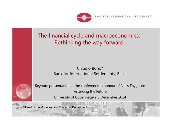
The financial cycle and macroeconomics: Rethinking the way forward Claudio Borio* Bank for International Settlements, Basel Keynote presentation at the conference in honour of Neils Thygesen Financing the Future University of Copenhagen, 5 December 2014 * Head of the Monetary and Economic Department.

Introduction Object of analysis:  • The financial cycle (FC), relationship with systemic financial crises (“financial distress” (FD)) and the business cycle (BC) • Analytical and policy implications FC = Self-reinforcing interaction between risk perceptions/tolerance and financing  constraints • can lead to widespread FD and macroeconomic dislocations • “procyclicality” of the financial system Basic thesis  • FC should be at the core of our understanding of the macroeconomy • Need to rethink approach to modelling Underlying themes: think medium term; think monetary; think global  Structure  • I - What is the FC? How is it related to financial crises and the BC? • II - What would it take to model it better? • III – Two illustrative implications of the analysis • Achilles heel of the international monetary and financial system (IMFS) • How to interpret the trend decline in real (natural?) interest rates 2

I. The FC: 7 key properties P1: Most parsimonious description: credit and property prices (G 1)  Equity prices can be a distraction  P2: The FC has a lower frequency (longer duration) than the traditional BC  (medium term!) 16-20 years approximately since 1980s (G 1)  - Traditional business cycle: up to 8 years P3: Peaks in the FC tend to coincide with FD (G 1)  Post-1985 all peaks do in sample of advanced economies examined  Few crises do not occur at peaks (all “imported”: cross-border exposures)  P4 : Risks of FD can be identified in real time with good lead (2-4 years)  (Private-sector) credit-to-GDP and asset prices (especially property prices) jointly  exceeding certain thresholds (G 2) - proxy for build-up of financial imbalances (FIs) Cross-border credit often outpaces domestic credit (G 3)  3

Graph 1 The financial and business cycles in the United States 0.15 Banking strains Financial crisis First oil crisis 0.10 Dotcom crash 0.05 0.00 –0.05 Second oil crisis Black Monday –0.10 –0.15 71 74 77 80 83 86 89 92 95 98 01 04 07 10 13 Financial cycle 1 Business cycle 2 1 The financial cycle as measured by frequency-based (bandpass) filters capturing medium-term cycles in real credit, the credit-to-GDP ratio and real house prices. 2 The business cycle as measured by a frequency-based (bandpass) filter capturing fluctuations in real GDP over a period from one to eight years. Source: updated from M Drehmann et al (2012) in BIS (2914). 4

Graph 2: Financial imbalances can be identified in real time The US example Credit-to-GDP gap Real property price gap Percentage points % The shaded areas refer to the threshold values for the indicators: 2–6 percentage points for credit-to-GDP gap; 15–25% for real property price gap. The estimates for 2008 are based on partial data (up to the third quarter). 1 Weighted average of residential and commercial property prices with weights corresponding to estimates of their share in overall property wealth. The legend refers to the residential property price component. Source: Borio and Drehmann (2009). 5

Graph 3: Credit booms and external credit: selected countries United States United Kingdom Thailand in the 1990s In billions of USD Incl cross-border credit to banks: Gross 2 9,000 300 21,000 Net 3 6,000 200 14,000 100 3,000 7,000 0 0 0 92 94 96 98 00 02 00 02 04 06 08 10 00 02 04 06 08 10 International Direct cross-border Credit credit 1 debt securities to non-financial private sector Year-on-year growth, in per cent 120 45 45 Including cross-border 90 30 30 Gross 2 credit to banks: Net 3 60 15 15 30 0 0 0 –15 –15 –30 –30 –30 92 94 96 98 00 00 02 04 06 08 10 00 02 04 06 08 10 Direct cross-border credit 1 The vertical lines indicate crisis episodes end-July 1997 for Thailand and end-Q2 2007 and end-Q3 2008 for the United States and the United Kingdom. Estimate of credit to the private non-financial sector granted by banks from offices located outside the country. 2 Estimate of credit as in footnote 1 1 plus cross-border borrowing by banks located in the country. 3 Estimate as in footnote (2) minus credit to non-residents granted by banks located in the country. Source: Borio et al (2011). 6

I. The FC: 7 key properties (ctd) P5: FC helps to measure potential (sustainable) output much better in real time  Current methods, partly based on inflation, can be very misleading (G 4)  P6 : Amplitude and length of the FC are regime-dependent: supported by  Financial liberalisation  - Weakens financing constraints MP frameworks focused on (near-term) inflation  - Provide less resistance to build-up Positive supply side developments (eg, globalisation of real economy)  - ↑ financial boom; ↓ inflation => “excess (financial) elasticity”  - Length and amplitude have increased since early 1980s (G 1) P7: Busts of FCs are associated with balance-sheet recessions (G 5)  Preceding boom is much longer  Debt and capital stock overhangs are much larger  Damage to financial sector is much greater  Policy room for manoeuvre is much more limited: buffers depleted  Result in permanent output losses  Usher in slow and long recoveries  - Japan; recent post-crisis recovery Why? Legacy of previous boom and subsequent financial strains  7

Graph 4 US output gaps: ex-post and real-time estimates In per cent of potential output IMF OECD 4 3 2 0 0 –3 –2 –6 –4 –9 –6 01 02 03 04 05 06 07 08 09 10 11 00 02 04 06 08 10 12 Finance neutral HP 3 3 0 0 –3 –3 –6 –6 –9 –9 01 02 03 04 05 06 07 08 09 10 11 01 02 03 04 05 06 07 08 09 10 11 Real-time Ex-post Note: For each time t, the “real-time” estimates are based only on the sample up to that point in time. The “ex-post” estimates are based on the full sample. Source: Borio et al (2013). 8

Graph 5: Balance sheet recessions are different 1 Monetary policy is less effective Deleveraging strengthens recovery Cyclically adjusted growth rate Cyclically adjusted growth rate during recovery during recovery 1 In per cent. The solid (dashed) regression lines indicate that the relationship is statistically significant (insignificant). For a sample of 24 economies since the mid- 1960s. Downturns are defined as periods of declining real GDP and recoveries as periods ending when real GDP exceeds the previous peak. The data cover 65 cycles, including 28 cycles with a financial crisis just before the peak. Data points for cycles are adjusted for the depth of the preceding recession and the interest rate at the cyclical peak. See Bech et al (2014) for details. Source: elaborated from Bech et al (2014) and included in BIS (2014). 9

II – What is needed to model the financial cycle? Features  The boom does not just precede but causes the bust  - endogenous financial and business cycles Meaningful treatment of capital stock and debt overhangs  - inclusion of stocks and disequilibria in stocks Potential output : distinguish ”non-inflationary” from ”sustainable” output  (G 4 above) - Concept and measurement How?  Endogenous time-varying risk perceptions/tolerance and defaults  - Limitations in expectations: expectations are not fully “rational” - Limitations in incentive: co-ordination failures A true monetary economy!  - Financial system does not just allocate “savings” but generates purchasing power • feeding back into output and expenditures - Inside money creation is essential - Current models are real economies disguised as monetary ones 10

II – Global C/A imbalances and the crisis: an example Global C/A imbalances did not play a significant role in the crisis  The “excess saving” view  Surplus countries “financed” the US credit boom  “Excess saving” reduced global (real) interest rates  Problem: conflates “financing” and “saving”  - Financing: (gross) cash flow concept - Saving: “hole” in aggregate demand ( ≡ investment) Expenditures need financing, not saving  - Credit important - Little relationship between credit and saving Objection 1 : Gross, not net, capital flows matter for financial stability  US credit boom was mostly financed domestically (Graph 4)  Foreign part mostly by European banks, including UK (balanced or deficit regions)  Objection 2 : Saving-investment balances affect natural, not market, interest rates  Monetary and financing conditions determine market rates  - expectations need not drive them to unobservable natural rate! - natural rate = equilibrium concept: can it cause a crisis? Little relationship: long-term rates and global saving or C/A balances (Graph 6)  Questionable application of “real” analysis to “monetary” economies  No distinction between saving and financing  11