The Fault of the Fed? The Fault of Fault of the the Fed Fed? ? - PowerPoint PPT Presentation

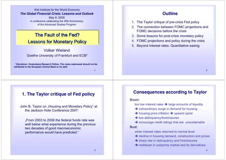
Kiel Institute for the World Economy Outline The Global Financial Crisis: Lessons and Outlook May 8, 2009 A conference celebrating the 25th Anniversary 1. The Taylor critique of pre-crisis Fed policy of the Advanced Studies Program 2. The connection between FOMC projections and FOMC decisions before the crisis The Fault of the Fed? The Fault of Fault of the the Fed Fed? ? The 3. Some lessons for post-crisis monetary policy Lessons for Monetary Policy Lessons for for Monetary Monetary Policy Policy 4. FOMC projections and policy during the crisis Lessons 5. Beyond interest rates: Quantitative easing Volker Wieland Goethe University of Frankfurt and ECB* * Disclaimer: Duisenberg Research Fellow. The views expressed should not be attributed to the European Central Bank or its staff. 1 2 Consequences according to Taylor 1. The Taylor critique of Fed policy Boom: too low interest rates � large amounts of liquidity John B. Taylor on „Housing and Monetary Policy“ at � extraordinary surge in demand for housing the Jackson Hole Conference 2007: � housing price inflation � upward spiral � low delinquency/foreclosures „From 2003 to 2006 the federal funds rate was � encourage credit ratings that are unsustainable well below what experience during the previous Bust: two decades of good macroeconomic when interest rates returned to normal level performance would have predicted.“ � decline in housing demand, construction and prices � sharp rise in delinquency and foreclosures � meltdown in subprime market and its derivatives. 3 4

Taylor‘s benchmark for comparison Poole‘s 2007 version of Taylor‘s rule A simple rule: = + π + π − π + − * * * f r 0.5( ) 0.5( y y ) t t t t t f: federal funds rate r*: real equilibrium rate π : inflation π *: inflation target y: real output y*: potential output William Poole (2007) (then-President of St.Louis Fed) ``The FOMC … views the Taylor rule as a general guideline. Departures from the rule make good sense when information beyond that incorporated in the rule is available.“ 5 6 Monetary policy and housing: Taylor‘s counterfactual Taylor‘s counterfactual � Effect on housing prices � Federal funds rates 7 8

Jarocinski & Smets 2008 The Jarocinski-Smets B-Var Forecasts from a B-VAR: � A Vector autoregression model in differences. It is specified in growth rates and uses Bayesian priors about the steady state. „These results suggest that the unusually low level of short-term and long-term interest rates (i,s) may have contributed to the boom in U.S. housing markets“. 9 10 Departures from the rule 2. FOMC projections and decisions � Humphrey-Hawkins report (February 2003) Poole (2007) � “ policy is forward looking; which means that from time to time the economic outlook changes sufficiently that it makes sense for the FOMC to set a funds rate either above or below the level called for in the Taylor rule which relies on observed recent data rather than on economic forecasts of future data.'' 11 12

Orphanides and Wieland (2008) July 2003 � Construct a time series of constant horizon (t+3 quarters) FOMC forecasts � from semi-annual Humphrey-Hawkins reports. � Estimate and compare forecast-based versus outcome-based policy rules. � Real-time outcomes from FRB Greenbook and ALFRED real time database. � Investigate whether FOMC projections help explain deviations from outcome-based Taylor rule. 13 14 FOMC projections – notation and data FOMC projections – notation and data � Time t in terms of quarters � 2 reports per year � semi-annual observations � Construct t+3 projections made in period t � February report: data can be used as is. u denotes unemployment, π denotes inflation. 15 16

Estimate forecast-based versus FOMC projections – notation and data outcome-based rules � July report: t+3 data needs to be constructed. � Specification estimated by non-linear least squares with data from 1988 to 2007: � Construct semi-annual inflation projections: � u: unemployment rate � Outcome-based: τ =t-1 � Forecast-based: τ =t+3 17 18 Regression results: 88-07 Actual Fed Funds vs Estimated Rules 19 No interest-rate smoothing, (1) and (3) in Table 1. 20

Rules with Smoothing But, FOMC Switched Inflation Measures! Examine Deviations � Changes in forecasts: � 2000:1 from consumer price index (CPI) to personal consumption expenditures price index (PCE) � 2004:2 from PCE to core PCE exluding food and energy � Possible implications for the rule: � Change in estimated coefficients? Therefore, re- estimate over CPI period. � Change in implied interest rates? Use other CPI forecasts in place of FOMC PCE forecasts. � What about forecast errors? With interest-rate smoothing, (2) and (4) in Table 1. 21 22 Extrapolation Using CPI Outcomes and Extrapolation 1988 – 2007 Bluechip CPI Forecasts Rule estimated with 1988-99 sample Uses FOMC preferred measures in terms of FOMC Projections as well as recent outcomes. 23 24

3. Some Lessons for Post-Crisis PCE Inflation: Actual vs Projected Monetary Policy Pretty big 5,6 forecast YES, Taylor has a point. It‘s awfully hard to claim error 4,8 that Fed policy had no role in the housing boom 4,0 and collapse that triggered the financial crisis, 3,2 AND, central banks should take simple rules more seriously. Deviations ought to be systematic 2,4 and well explained. 1,6 DON‘T rely too much on forecasts, particularly if 0,8 those measures may be revised substantially. 0,0 1988 1989 1990 1991 1992 1993 1994 1995 1996 1997 1998 1999 2000 2001 2002 2003 2004 2005 2006 2007 FOMC Projections PCE Compares real-time FOMC projections to outcomes 25 26 as measured using the July 2007 vintage data. 4. FOMC projections and decisions Lessons cont‘d during the financial crisis AND NO, it is not yet self-evident that central � Starting in October 2007 the FOMC has been banks should respond to asset prices directly publishing projections on a quarterly basis. over and above output and inflation. � Inflation measures include PCE and core PCE, AND, it is not necessary to fix exchange rates or but not CPI. return to the gold standard. � The horizon has been extended. Central banks should remain independent and in � We apply the rule estimated in Orphanides and charge of interest rate policy, with more weight Wieland (2008) to generate interest rate given to simple rules than sophisticated predictions based on the new quarterly FOMC discretion. projections data. 27 28

Extrapolation with 2007-09 projections The January 2009 Outlook 6,0 5,0 4,0 3,0 2,0 Preemptive Easing 1,0 0,0 2005:Q4 2006:Q1 2006:Q2 2006:Q3 2006:Q4 2007:Q1 2007:Q2 2007:Q3 2007:Q4 2008:Q1 2008:Q2 2008:Q3 2008:Q4 2009:Q1 2009:Q2 -1,0 -2,0 -3,0 Negative Rates - Quantitative Easing -4,0 -5,0 Federal Runds Rate Forecast-based Rule (no smooth.) 29 30 Forecast-based Rule (with smooth) Aggressiveness depends a lot on Risk-Premia Offset vs. Preemptive Easing response to unemployment 6,0 6,0 5,0 5,0 4,0 4,0 3,0 3,0 Coefficient on deviations of u Preemptive easing 2,0 2,0 from u* halfed, u* = 4.9 smaller if risk premia 1,0 1,0 considered 0,0 0,0 2005:Q4 2006:Q1 2006:Q2 2006:Q3 2006:Q4 2007:Q1 2007:Q2 2007:Q3 2007:Q4 2008:Q1 2008:Q2 2008:Q3 2008:Q4 2009:Q1 2009:Q2 2005:Q4 2006:Q1 2006:Q2 2006:Q3 2006:Q4 2007:Q1 2007:Q2 2007:Q3 2007:Q4 2008:Q1 2008:Q2 2008:Q3 2008:Q4 2009:Q1 2009:Q2 -1,0 -1,0 -2,0 -2,0 -3,0 -3,0 -4,0 -4,0 -5,0 -5,0 Federal Runds Rate Forecast-based Rule (with smooth) adjusted Federal Runds Rate 3-Month LIBOR Forecast-based Rule (no smooth.) 31 32 Forecast-based Rule (with smooth) 3-Month LIBOR

5. Beyond interest rates: Quantitative easing Quantitative easing � Orphanides and Wieland (2000), Coenen and Does quantitative easing have any real effects? Wieland (2003): � Direct effects of money on demand and inflation, (real balance and portfolio-balance effects) still � Usually monetary policy is conducted via open remain active at zero-interest rate floor. market operations but with an operating target for the money market rate. � The effect of an increase in the monetary base is smaller than in normal times and estimates are � Taylor-rule style monetary policy may be re- rather imprecise. formulated as a rule in terms of the monetary base. � May justify pre-emptive interest rate reduction and � When rate is at zero-interest rate floor, central aggressive quantitative easing. bank can continue with direct purchases of assets (government debt , private sector debt) and/ or longer-term operations in the money market. 33 34 Policy as a base money rule Zero bound on policy interest rate Effect of monetary expansion is � m = base money / (price level * real income) Interest reduced when zero rate, � Base money rule in normal times ( f> 0), similar interest rate bound Monetary is hit. to interest rate rule but not as practical. base = − π π − π − − * * m k ( ) k ( y y ) t t y t t � Base money rule at zero-interest floor ( f=0), 0 magnification factor x. = − π π − π − − * * m xk ( ) xk ( y y ) t t y t t Underlying 0 inflation 35 36