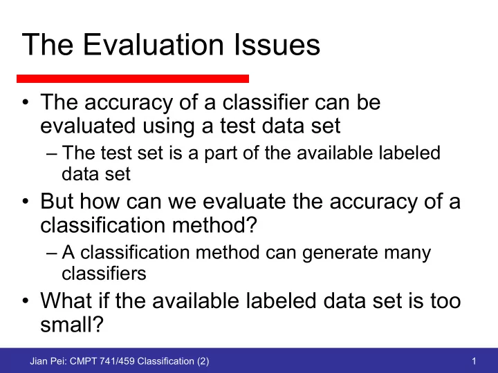
The Evaluation Issues The accuracy of a classifier can be evaluated - PowerPoint PPT Presentation

The Evaluation Issues • The accuracy of a classifier can be evaluated using a test data set – The test set is a part of the available labeled data set • But how can we evaluate the accuracy of a classification method? – A classification method can generate many classifiers • What if the available labeled data set is too small? Jian Pei: CMPT 741/459 Classification (2) 1

Holdout Method • Partition the available labeled data set into two disjoint subsets: the training set and the test set – 50-50 – 2/3 for training and 1/3 for testing • Build a classifier using the training set • Evaluate the accuracy using the test set Jian Pei: CMPT 741/459 Classification (2) 2

Limitations of Holdout Method • Fewer labeled examples for training • The classifier highly depends on the composition of the training and test sets – The smaller the training set, the larger the variance • If the test set is too small, the evaluation is not reliable • The training and test sets are not independent Jian Pei: CMPT 741/459 Classification (2) 3

Cross-Validation • Each record is used the same number of times for training and exactly once for testing • K-fold cross-validation – Partition the data into k equal-sized subsets – In each round, use one subset as the test set, and use the rest subsets together as the training set – Repeat k times – The total error is the sum of the errors in k rounds • Leave-one-out: k = n – Utilize as much data as possible for training – Computationally expensive Jian Pei: CMPT 741/459 Classification (2) 4

Confidence Interval for Accuracy • Suppose a classifier C is tested on a test set of n cases, and the accuracy is acc • How much confidence can we have on acc? • We need to estimate the confidence interval of a given model accuracy – Within which one is sufficiently sure that the true population value lies or, equivalently, by placing a bound on the probable error of the estimate • A confidence interval procedure uses the data to determine an interval with the property that – viewed before the sample is selected – the interval has a given high probability of containing the true population value Jian Pei: CMPT 741/459 Classification (2) 5

Binomial Experiments • When a coin is flipped, it has a probability p to have the head turned up • If the coin is flipped N times, what is the probability that we see the head X times? – Expectation (mean): Np – Variance: Np(1 - p) N ⎛ ⎞ v N v P ( X v ) p ( 1 p ) − ⎜ ⎟ = = − ⎜ ⎟ v ⎝ ⎠ Jian Pei: CMPT 741/459 Classification (2) 6

Confidence Level and Approximation Area = 1 - α acc p − P ( Z Z ) < < p ( 1 p ) / N / 2 1 / 2 α − α − 1 = − α Approximating using normal distribution Z α : the bound at confidence level (1- α ) Z α /2 Z 1- α /2 2 2 2 2 N acc Z Z Z 4 N acc 4 N acc ⋅ + ± + ⋅ − ⋅ / 2 / 2 / 2 α α α 2 2 ( N Z ) + / 2 α Jian Pei: CMPT 741/459 Classification (2) 7

Accuracy Can Be Misleading … • Consider a data set of 99% of the negative class and 1% of the positive class • A classifier predicts everything negative has an accuracy of 99%, though it does not work for the positive class at all! • Imbalance class distribution is popular in many applications – Medical applications, fraud detection, … Jian Pei: CMPT 741/459 Classification (2) 8

Performance Evaluation Matrix Confusion matrix (contingency table, error matrix): used for imbalance class distribution PREDICTED CLASS Class=Yes Class=No ACTUAL Class=Yes a (TP) b (FN) CLASS Class=No c (FP) d (TN) a d TP TN + + Accuracy = = a b c d TP TN FP FN + + + + + + Jian Pei: CMPT 741/459 Classification (2) 9

Performance Evaluation Matrix PREDICTED CLASS Class=Yes Class=No ACTUAL Class=Yes a (TP) b (FN) CLASS Class=No c (FP) d (TN) True positive rate (TPR, sensitivity) = TP / (TP + FN) True negative rate (TNR, specificity) = TN / (TN + FP) False positive rate (FNR) = FP / (TN + FP) False negative rate (FNR) = FN / (TP + FN) Jian Pei: CMPT 741/459 Classification (2) 10

Recall and Precision • Target class is more important than the other classes PREDICTED CLASS Class=Yes Class=No ACTUAL Class=Yes a (TP) b (FN) CLASS Class=No c (FP) d (TN) Precision p = TP / (TP + FP) Recall r = TP / (TP + FN) Jian Pei: CMPT 741/459 Classification (2) 11

Fallout • Type I errors – false positive: a negative object is classified as positive – Fallout: the type I error rate, FP / (TP + FP) • Type II errors – false negative: a positive object is classified as negative – Captured by recall Jian Pei: CMPT 741/459 Classification (2) 12

F β Measure • How can we summarize precision and recall into one metric? – Using the harmonic mean between the two 2 rp 2 TP F - measure (F) = = r p 2 TP FP FN + + + • F β measure β = ( β 2 + 1) rp ( β 2 + 1) TP F r + β 2 p = ( β 2 + 1) TP + β 2 FN + FP – β = 0, F β is the precision – β = ∞ , F β is the recall – 0 < β < ∞ , F β is a tradeoff between the precision and the recall Jian Pei: CMPT 741/459 Classification (2) 13

Weighted Accuracy • A more general metric w a w d + Weighted Accuracy = 1 4 w a w b w c w d + + + 1 2 3 4 Measure w1 w2 w3 w4 Recall 1 1 0 0 Precision 1 0 1 0 F β β 2 + 1 β 2 1 0 Accuracy 1 1 1 1 Jian Pei: CMPT 741/459 Classification (2) 14

ROC Curve • Receiver Operating Characteristic (ROC) 1-dimensional data set containing 2 classes. Any points located at x > t is classified as positive Jian Pei: CMPT 741/459 Classification (2) 15

ROC Curve (TP,FP): • (0,0): declare everything to be negative class • (1,1): declare everything to be positive class • (1,0): ideal • Diagonal line: – Random guessing – Below diagonal line: prediction is opposite of the true class Figure from [Tan, Steinbach, Kumar] Jian Pei: CMPT 741/459 Classification (2) 16

Comparing Two Classifiers Figure from [Tan, Steinbach, Kumar] Jian Pei: CMPT 741/459 Classification (2) 17

Cost-Sensitive Learning • In some applications, misclassifying some classes may be disastrous – Tumor detection, fraud detection • Using a cost matrix PREDICTED CLASS Class=Yes Class=No ACTUAL Class=Yes -1 100 CLASS Class=No 1 0 Jian Pei: CMPT 741/459 Classification (2) 18

Sampling for Imbalance Classes • Consider a data set containing 100 positive examples and 1,000 negative examples • Undersampling: use a random sample of 100 negative examples and all positive examples – Some useful negative examples may be lost – Run undersampling multiple times, use the ensemble of multiple base classifiers – Focused undersampling: remove negative samples that are not useful for classification, e.g., those far away from the decision boundary Jian Pei: CMPT 741/459 Classification (2) 19

Oversampling • Replicate the positive examples until the training set has an equal number of positive and negative examples • For noisy data, may cause overfitting Jian Pei: CMPT 741/459 Classification (2) 20

Significance Tests • Are two algorithms different in effectiveness? – The null hypothesis: there is NO difference – The alternative hypothesis: there is a difference – B is better than A (the baseline method) • Matched pair experiments: the rankings that are compared are based on the same set of queries for both algorithms • Possible errors of significant tests – Type I: the null hypothesis is rejected when it is true – Type II: the null hypothesis is accepted when it is false • The power of a hypothesis test: the probability that the test will reject the null hypothesis correctly – Reducing the type II errors Jian Pei: CMPT 741/459 Classification (2) 21

Procedure of Comparison • Using a set of data sets • Procedure – Compute the effectiveness measure for every data set – Compute a test statistic based on a comparison of the effectiveness measures for each data set • E.g., the t-test, the Wilcoxon signed-rank test, and the sign test – Compute a P-value: the probability that a test statistic value at least that extreme could be observed if the null hypothesis were true – The null hypothesis is rejected if the P-value ≤ α , where α is the significance level which is used to minimize the type I errors • One-sided (one-tailed) tests: whether B is better than A (the baseline method) – Two-sided tests: whether A and B are different – the P-value is doubled Jian Pei: CMPT 741/459 Classification (2) 22

Distribution of Test Statistics Jian Pei: CMPT 741/459 Classification (2) 23

T-test • Assuming data values are sampled from normal distributions – In a matched pair experiment, assuming the difference between the effectiveness values is a sample from a normal distribution • The null hypothesis: the mean of the distribution of difference is 0 B A − t N = σ B − A – B – A is the mean of the differences, σ B – A is the standard deviation of the differences 1 N 2 2 ( x x ) ∑ σ = − i N i 1 = Jian Pei: CMPT 741/459 Classification (2) 24

Example B A 21 . 4 − = 29 . 1 σ = B A − t 2 . 33 = P-value = 0.02 significant at a level of σ = 0.05 – the null hypothesis can be rejected Jian Pei: CMPT 741/459 Classification (2) 25