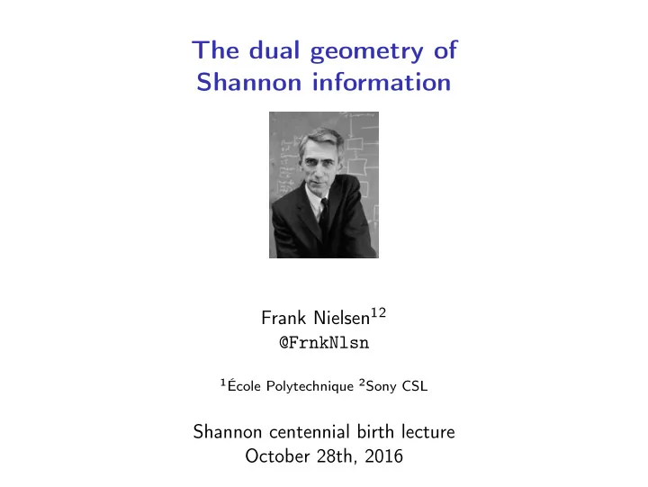
The dual geometry of Shannon information Frank Nielsen 12 @FrnkNlsn - PowerPoint PPT Presentation

The dual geometry of Shannon information Frank Nielsen 12 @FrnkNlsn 1 École Polytechnique 2 Sony CSL Shannon centennial birth lecture October 28th, 2016

Outline A storytelling... ◮ Getting started with the framework of information geometry: 1. Shannon entropy and satellite concepts 2. Invariance and information geometry 3. Relative entropy minimization as information projections ◮ Recent work overview: 4. Chernoff information and Voronoi information diagrams 5. Some geometric clustering in information spaces 6. Summary of statistical distances with their properties ◮ Closing: Information Theory onward 1

Chapter I. Shannon entropy and satellite concepts 2

Shannon entropy (1940’s): Big bang of IT! ◮ Discrete entropy : probability mass function (pmf) p i = P ( X = x i ) , x i ∈ X (0 log 0 = 0) p i log 1 � � H ( X ) = = − p i log p i p i i = 1 i = 1 ◮ Differential entropy : probability density function (pdf) X ∼ p with support X � h ( X ) = − p ( x ) log p ( x ) d x X ◮ Probability measure: random variable X ∼ P ≪ µ � log d P H ( X ) = − d µ d P X � p = d P H ( X ) = − p ( x ) log p ( x ) d µ ( x ) , d µ X Lebesgue measure µ L , counting measure µ c , 3

Discrete vs differential Shannon entropy Entropy: Measure the (expected) uncertainty of a random variable (rv) � H ( X ) = − p ( x ) log p ( x ) d µ ( x ) = − E X [ log X ] , X ∼ P X ◮ Discrete entropy is bounded : 0 ≤ H ( X ) ≤ log |X| with support X ◮ Differential entropy... ◮ may be negative : H ( X ) = 1 2 log ( 2 π e σ 2 ) , X ∼ N ( µ, σ ) for Gaussians ◮ may be infinite when integral diverges: H ( X ) = ∞ log ( 2 ) X ∼ p ( x ) = x log 2 x for x > 2, with support X = ( 2 , ∞ ) 4

Key property: Shannon entropy is concave... Graph plot of Shannon binary entropy (H of Bernoulli trial): X ∼ Bernoulli ( p ) with p = Pr ( X = 1 ) H ( X ) = − ( p log p + ( 1 − p ) log ( 1 − p )) ... and Shannon information − H ( X ) (neg-entropy) is convex 5

Maximum entropy principle (Jaynes [12], 1957): Exponential families (Gibbs distribution) ◮ A finite set of D moment (expectation) constraints t i : E p ( x ) [ t i ( X )] = η i for i ∈ [ D ] = { 1 , . . . , D } ◮ Solution (Lagrangian multipliers): = Exponential Family [34] p ( x ) = p ( x ; θ ) = exp ( � θ, t ( x ) � − F ( θ )) where � a , b � = a ⊤ b : dot/scalar/inner product. ◮ MaxEnt : max θ H ( p ( x ; θ )) such that E p ( x ; θ ) [ t ( X )] = η , t ( x ) = ( t 1 ( x ) , . . . , t D ( x )) and η = ( η 1 , . . . , η D ) ◮ Consider a parametric family { p ( x ; θ ) } θ ∈ Θ , θ ∈ R D , D : order 6

Exponential families (EFs) [34] ◮ Log-normalizer (cumulant, partition function, free energy): �� � � exp ( � θ, t ( x ) � ) d ν ( x ) ← F ( θ ) = log p ( x ; θ ) d ν ( x ) = 1 Here, F strictly convex , here C ∞ . p ( x ; θ ) = e � θ, t ( x ) �− F ( θ ) ◮ Natural parameter space: Θ = { θ ∈ R D : F ( θ ) < ∞} ◮ EFs have all finite order moments expressed using the Moment Generating Function (MGF): M ( u ) = E [ exp ( � u , X � )] = exp ( F ( θ + u ) − F ( θ )) E [ t ( X ) l ] = M ( l ) ( 0 ) Geometric moments: for order D = 1 V [ t ( X )] = ∇ 2 F ( θ ) ≻ 0 E [ t ( X )] = ∇ F ( θ ) = η, 7

Example: MaxEnt distribution with fixed mean and fixed variance = Gaussian family ◮ max p H ( p ( x )) = max θ H ( p ( x ; θ )) such that: E p ( x ; θ ) [ X ] = η 1 (= µ ) , η 2 (= µ 2 + σ 2 ) E p ( x ; θ ) [ X 2 ] = Indeed, V p ( x ; θ ) [ X ] = E [( X − µ ) 2 ] = E [ X 2 ] − µ 2 = σ 2 ◮ Gaussian distribution is maxent distribution: � � 2 � � x − µ 1 − 1 = e � θ, t ( x ) �− F ( θ ) √ p ( x ; θ ( µ, σ )) = exp 2 σ σ 2 π ◮ sufficient statistic vector: t ( x ) = ( x , x 2 ) ◮ natural parameter vector: θ = ( θ 1 , θ 2 ) = ( µ σ 2 , − 1 2 σ 2 ) � � ◮ log-normalizer: F ( θ ) = − θ 2 4 θ 2 + 1 − π 2 log 1 θ 2 ◮ By construction, E [ t ( x ) = ( x , x 2 )] = ∇ F ( θ ) = η = ( µ, µ 2 + σ 2 ) 8

Entropy of an EF and convex conjugates X ∼ p ( x ; θ ) = exp ( � θ, t ( x ) � − F ( θ )) , E p ( x ; θ ) [ t ( X )] = η ◮ Entropy of an EF: � H ( X ) = − p ( x ; θ ) log p ( x ; θ ) = F ( θ ) − � θ, η � ◮ Legendre convex conjugates [20]: F ∗ ( η ) = − F ( θ ) + � θ, η � ◮ H ( X ) = F ( θ ) − � θ, η � = − F ∗ ( η ) < ∞ (always finite here!) ◮ A member of an exponential family can be canonically parameterized either by using its natural parameter θ = ∇ F ∗ ( η ) or by using its expectation parameter η = ∇ F ( θ ) , see [34] ◮ Converting η -to- θ parameters can be seen as a MaxEnt optimization problem. Rarely in closed-form! 9

MaxEnt and Kullback-Leibler divergence ◮ Statistical distance : Kullback-Leibler divergence Aka. relative entropy, P , Q ≪ µ , p = d P d µ , q = d Q d µ � p ( x ) log p ( x ) KL ( P : Q ) = q ( x ) d µ ( x ) ◮ KL is not a metric distance: asymmetric and does not satisfy triangle inequality ◮ KL ( P : Q ) ≥ 0 (Gibb’s inequality) and KL may be infinite : 1 p ( x ) = π ( 1 + x 2 ) = Cauchy distribution 2 π exp ( − x 2 1 2 ) = standard normal distribution q ( x ) = √ KL ( p : q ) = + ∞ diverges while KL ( q : p ) < ∞ converges. 10

MaxEnt as a convex minimization program ◮ Maximizing concave entropy H under linear moment constraints ≡ minimizing convex information ◮ MaxEnt ≡ convex minimization with linear constraints (the t i ( x j ) are prescribed constants) � min p j log p j (CVX) p ∈ ∆ D + 1 j � constraints: p j t i ( x j ) = η j , ∀ i ∈ [ D ] j p j ≥ 0 , ∀ i ∈ [ |X| ] � p j = 1 j ∆ D + 1 : D -dimensional probability simplex, embedded in R D + 1 + 11

MaxEnt with prior and general canonical EF MaxEnt H ( P ) ≡ left-sided min P KL ( P : U ) wrt U U : uniform distribution H ( U ) = log |X| . max P H ( P ) = log |X| − min P KL ( P : U ) with KL amounting to “cross-entropy minus entropy”: � � 1 1 KL ( P : Q ) = p ( x ) log q ( x ) d x − p ( x ) log p ( x ) d x � �� � � �� � H × ( P : Q ) H ( p )= H × ( P : P ) ◮ Generalized MaxEnt problem : Minimize KL distance to prior distribution h under constraints (MaxEnt is recovered when h = U , uniform distribution) min p KL ( p : h ) � constraints: p j t i ( x j ) = η j , ∀ i ∈ [ D ] j � p j ≥ 0 , ∀ i ∈ [ |X| ] , p j = 1 12 j

Solution of MaxEnt with prior distribution ◮ General canonical form of exponential families (using Lagrange multipliers for constrained optimization) p ( x ; θ ) = exp ( � θ, t ( x ) � − F ( θ )) h ( x ) ◮ Since h ( x ) > 0, let h ( x ) = exp ( k ( x )) for k ( x ) = log h ( x ) ◮ Exponential families are log-concave ( F is convex): l ( x ; θ ) = log p ( x ; θ ) = � θ, t ( x ) � − F ( θ ) + k ( x ) ◮ Entropy of general EF [37]: H ( X ) = − F ∗ ( η ) − E [ k ( x )] X ∼ p ( x ; θ ) , ◮ many common distributions [34] p ( x ; λ ) are EFs with θ = θ ( λ ) and carrier distribution d ν ( x ) = e k ( x ) d µ ( x ) (eg., Rayleigh) 13

Maximum Likelihood Estimator (MLE) for EFs ◮ Given observations S = { s 1 , . . . , s m } ∼ iid p ( x ; θ 0 ) , MLE: � ˆ θ m = argmax θ L ( θ ; S ) = p ( s i ; θ ) i argmax θ l ( θ ; S ) = 1 � ≡ l ( s i ; θ ) m i ◮ “Normal equation” of MLE [34]: m θ m ) = 1 � η m = ∇ F (ˆ ˆ t ( s i ) m i = 1 ◮ MLE problem is linear in η but convex in θ : � 1 � � min θ F ( θ ) − i t ( s i ) , θ m ◮ MLE is consistent : lim m →∞ ˆ θ m = θ 0 η m ) + 1 � ◮ Average log-likelihood [23]: l (ˆ θ m ; S ) = F ∗ (ˆ i k ( s i ) m 14

MLE as a right-sided KL minimization problem � m ◮ Empirical distribution: p e ( x ) = 1 i = 1 δ s i ( x ) . m Powerful modeling: data and models coexist in the space of distributions p e ≪ p ( x ; θ ) is absolutely continuous with respect to p ( x ; θ ) min KL ( p e ( x ) : p θ ( x ) ) � � p e ( x ) log p e ( x ) d x − = p e ( x ) log p θ ( x ) d x = min − H ( p e ) − E p e [ log p θ ( x )] � �� � ≡ max 1 � δ ( x − x i ) log p θ ( x ) n max 1 � = log p θ ( x i ) = MLE n i ◮ Since KL ( p e ( x ) : p θ ( x )) = H × ( p e ( x ) : p θ ( x )) − H ( p e ( x )) , min KL ( p e ( x ) : p θ ( x )) amounts to minimize the cross-entropy 15

Fisher Information Matrix (FIM) and CRLB [24] ∂ Notation: ∂ i l ( x ; θ ) = ∂θ i l ( x ; θ ) ◮ Fisher Information Matrix (FIM) : I ( θ ) � 0 I = [ I i , j ] ij , I i , j ( θ ) = E θ [ ∂ i l ( x ; θ ) ∂ j l ( x ; θ )] , ◮ Cramér-Rao/Fréchet lower bound (CRLB) for an unbiased estimator ˆ θ m with θ 0 optimal parameter (hidden by nature): V [ˆ θ m ] � I − 1 ( θ 0 ) , V [ˆ θ m ] − I − 1 ( θ 0 ) is PSD ◮ efficiency : unbiased estimator matching the CR lower bound ◮ asymptotic normality of MLE ˆ θ (on random vectors): � � θ 0 , 1 mI − 1 ( θ 0 ) ˆ θ m ∼ N 16