Texturing Graphics & Visualization: Principles & Algorithms - PowerPoint PPT Presentation
Graphics & Visualization Chapter 14 Texturing Graphics & Visualization: Principles & Algorithms Chapter 14 Texturing Why? On every surface, the human visual system can detect: Small
Texture Mapping Polygonal Surfaces (4) • Bilinear coordinate interpolation is possible: when progressively sampling the polygon surface in a regular manner or when the surface- and texture-coordinate parameterizations are coincident • Bilinear coordinate interpolation is not convenient if: single texture-coordinate sample is required at an arbitrary location on a triangle We can use the barycentric coordinate representation of the triangle instead 20 Graphics & Visualization: Principles & Algorithms Chapter 14
Barycentric Coordinates • Any point p on a triangle p 1 p 2 p 3 plane can be represented as an affine combination of those 3 basis points: (14.4) p = p + p + p , 1 1 2 2 3 3 • Parametric domain is a plane in 3 • By restricting λ 1 , λ 2 , λ 3 to [0,1] barycentric triangle form of (14.4) becomes a function that maps an equilateral triangle in space to a range that is exactly the interior of the triangle p 1 p 2 p 3 21 Graphics & Visualization: Principles & Algorithms Chapter 14
Barycentric Coordinates (2) • The 3 barycentric coordinates are directly associated with the ratios of the triangle areas formed by point p to the total : A A ( p p p ) , 1 2 3 1 A A ( p p p ) 1 2 3 (14.6) A ( p p p ) , A 1 3 2 2 A A ( p p p ) 1 2 3 A A ( p p p ) 3 1 2 1 , 3 1 2 A A ( p p p ) 1 2 3 where A( v 1 , v 2 , v 3 ) is the area of triangle v 1 v 2 v 3 22 Graphics & Visualization: Principles & Algorithms Chapter 14
Barycentric Coordinates (3) • Calculation of the barycentric triangle coordinates from ratios of triangle areas: • Since area of a triangle is proportional to the magnitude of the cross product of 2 of its edges A ( v v v ) v v v v / 2, 1 2 3 1 2 1 3 barycentric coordinates can be calculated by transforming (14.6) to: pp pp p p p p 2 3 1 1 3 (14.7) , , 1 1 2 3 1 2 p p p p p p p p 1 2 1 3 1 2 1 3 23 Graphics & Visualization: Principles & Algorithms Chapter 14
Barycentric Coordinates (4) • Texture coordinates ( u , v ) for point p can be easily interpolated from the texture coordinates ( u i , v i ), i =1 … 3 stored in the vertex data of p 1 p 2 p 3 : u u u u , 1 1 2 2 3 3 (14.8) v v v v . 1 1 2 2 3 3 • Parameter-interpolation is more generic than bilinear interpolation BUT more costly to perform should be used when a progressive scan is not possible 24 Graphics & Visualization: Principles & Algorithms Chapter 14
Texture-Coordinate Generation • u , v parameters have been deduced from the Cartesian coordinates of the vertices with the help of a texture- coordinate generation function: Provides a simple mapping from the Cartesian domain to the bounded normalized domain in texture space • Most common functions perform the mapping in 2 steps: Arbitrary Cartesian coordinates predetermined “auxiliary” surface embedded in space (shape represented parametrically) Auxiliary surface parameters are normalized to represent texture coordinates 25 Graphics & Visualization: Principles & Algorithms Chapter 14
Texture-Coordinate Generation (2) • The parametric surface determines how a planar textured sheet is wrapped around the original object • Important issue: Tiling Texture-coordinate generation transformation should map a point in space into the bounded domain of the image map: [0,1] [0,1] • For texture coordinate estimation for polygons, wrapping to [0,1] must be performed after the interpolation of the values during rasterization 26 Graphics & Visualization: Principles & Algorithms Chapter 14
Texture-Coordinate Generation (3) • If a texture parameter is wrapped to the [0,1] range before assigned to a vertex interpolated values between 2 consecutive vertices can be accidentally reversed: 27 Graphics & Visualization: Principles & Algorithms Chapter 14
Texture-Coordinate Generation (4) • The 2 most common local attributes used for texture-coordinate generation: Location in space of the fragment being rendered Local surface normal vector • Other local attributes can be exploited in order to address the texture space (i.e. incident-light direction) 28 Graphics & Visualization: Principles & Algorithms Chapter 14
Planar Mapping • Planar Mapping: Simplest ( u , v )-coordinate generation function Uses a plane as an intermediate parametric surface Cartesian coordinates are parallelly projected onto the plane u x x x a x · offset , v y y y b y · offset (14.9) x y Although an arbitrary plane can be used, selecting one that is axis-aligned greatly simplifies the calculations 29 Graphics & Visualization: Principles & Algorithms Chapter 14
Planar Mapping (2) • Planar mapping using the xy -plane. Note that all points with the same x,y -coordinates are mapped onto the same texture-map location 30 Graphics & Visualization: Principles & Algorithms Chapter 14
Planar Mapping (3) • In Equation (14.9), a , b are the tiling factors and ( offset x , offset y ) is the offset from the lower-left corner of the image in texture- coordinate space • Tiling factors determine how many repetitions of the texture image should fit in one world-coordinate-system unit • Planar mapping is useful for texturing flat surface regions that can be represented in a functional manner, as in z = f ( x , y ) • The more parallel a surface region is to the projection plane, the less distorted the projected texture is. 31 Graphics & Visualization: Principles & Algorithms Chapter 14
Cylindrical Mapping • Cylindrical Mapping: Texture coordinates are derived from the cylindrical coordinates of a point p in space: 1 tan ( / ), x z (14.10) h y , 2 2 ( ) r x z where θ is the right-handed angle from the z - to x -axis, with - π < θ ≤ π , h is the vertical offset from the xz -plane, & r is the distance of p from the y -axis • ( u , v )-coordinates can be associated with any 2 of the cylindrical coordinates of Equation (14.10): Usually u is derived from θ & v is calculated from the height h 32 Graphics & Visualization: Principles & Algorithms Chapter 14
Cylindrical Mapping (2) • The result of cylindrical mapping is similar to wrapping a photograph around an infinitely long tube: • All points with the same bearing and height are mapped to the same point in texture space for all r [0 ,∞) 33 Graphics & Visualization: Principles & Algorithms Chapter 14
Cylindrical Mapping (3) • Cylindrical coordinates of Equation (14.10) can be easily transformed into texture coordinates using: 1 1 1 tan ( / ) , x z u (14.11) 2 2 2 2 v h y • Above formulation of the ( u , v )-coordinate pair can be augmented to include the tiling factors a & b around & along the y -axis, respectively: a ( ) , a u (14.12) 2 2 v by by 34 Graphics & Visualization: Principles & Algorithms Chapter 14
Spherical Mapping • Spherical Mapping: Texture-coordinate generation function depends on the spherical coordinates ( θ , φ , r ) of a point in space • θ is the longitude of the point, φ is the latitude and r is the distance from the coordinate system origin • Spherical coordinates of a point p = ( x , y , z ) are given by: x 1 tan z y (14.13) 1 tan 2 2 2 2 x z 2 2 2 r x y z 35 Graphics & Visualization: Principles & Algorithms Chapter 14
Spherical Mapping (2) • Spherical mapping: (a) The texture-coordinate parameterization and image wrapping (b) An evening-sky texture mapped to a dome using the spherical texture-coordinate generation function 36 Graphics & Visualization: Principles & Algorithms Chapter 14
Spherical Mapping (3) • Spherical texture-coordinate generation usually associates the u - & v -coordinates with the 2 angular components of the above representation: / 2 (14.14) u , v 2 • Using a pair of tiling factors ( a , b ) for the u - & v - coordinates, respectively, the spherical mapping is given by: a a (14.15) u , 2 2 b / 2 b / 2 v 37 Graphics & Visualization: Principles & Algorithms Chapter 14
Spherical Mapping (4) • Spherical mapping operation wraps an image around an object like a world atlas maps to the globe • Spatial resolution of a texel varies according to the latitude of the point heavy distortion at the poles: a whole line of the texture is typically mapped onto a single point in space 38 Graphics & Visualization: Principles & Algorithms Chapter 14
Spherical Mapping (5) • For calculation of the texture parameters, normal vector coordinates can be used instead of the point location: Replace ( x , y , z ) point coordinates of Equation (14.13) with the normal vector components ( n x , n y , n z ) Uses: • Pre-calculate, store and index incoming diffuse illumination from distant light sources as texture map • Replace the Phong model with any (e.g. toon shading) precalculated spherical function and apply as texture Light sources are considered to be infinitely far from the objects 39 Graphics & Visualization: Principles & Algorithms Chapter 14
Cube (Box) Mapping • Combines local surface-direction information with the Cartesian coordinates of the point derive the texture coordinates • One of the 3 primary axes is selected according to the principal normal direction component • A point p is projected onto plane xy , yz , or xz , depending on whether the absolute value of the z -, x -, or y -coordinate, of the normal vector is the largest one • Planar mapping for each one of the 3 cases properly substituting the coordinate pairs in Equation (14.9) 40 Graphics & Visualization: Principles & Algorithms Chapter 14
Cube Mapping (2) • Cube mapping is ideal for multifaceted geometry & for shapes with right angles • Useful property: Texture map is never projected on a surface from an angle of more than 45 degrees from the surface normal 41 Graphics & Visualization: Principles & Algorithms Chapter 14
Cube Mapping (3) • We get no significant distortion from texel stretching but • Transition from one projection plane to another is prone to causing discontinuities 42 Graphics & Visualization: Principles & Algorithms Chapter 14
Cube Mapping Why use this mapping paradigm? • In spherical mapping significant distortion at the poles is caused due to the inherent mapping singularity • Cube mapping avoids this pitfall by always selecting the side of a cube that is most perpendicular to the vector associated with the current point • 6 maps are prepared and indexed instead of 1 43 Graphics & Visualization: Principles & Algorithms Chapter 14
Cube Mapping Example • Cube mapping using vector coordinates to apply pre-calculated diffuse illumination to an object: (a) Set-up (b) 6 cube maps (c) Texture-shaded object in its final environment 44 Graphics & Visualization: Principles & Algorithms Chapter 14
Cube Mapping Calculations • Cube-mapping texture coordinates are calculated as the normalized coordinates in the range [0,1] of a vector v ( v v v , , ) x y z • Appropriate cube texture is selected according to the largest-in-magnitude signed component of the vector provided • Cube mapping on vector coordinates is implemented both in OpenGL and Direct3D in a consistent manner 45 Graphics & Visualization: Principles & Algorithms Chapter 14
Cube Mapping Calculations (2) 1 ( u c 1), u 2 m a (14.16) 1 ( v c v 1) 2 m a where: ( u v m , , ) ( v , v v , ) v max{ v , v , v }, c c a z y x x x y z ( , , ) ( , , ) max{ , , }, u v m v v v v v v v c c a z y x x x y z ( u v m , , ) ( v v v , , ) v max{ v , v , v }, c c a x z y y x y z (14.17) ( u v m , , ) ( v , v v , ) v max{ v , v , v }, c c a x z y y x y z ( u v m , , ) ( v , v v , ) v max{ v , v , v }, c c a x y z z x y z ( u v m , , ) ( v , v v , ) v max{ v , v , v }. c c a x y z z x y z 46 Graphics & Visualization: Principles & Algorithms Chapter 14
The Use of Cube Mapping • Cube mapping is very frequently used for representing 3-D environment extents, such as: distant landscapes, buildings in cityscapes, sky boxes, and sky domes • When the interpolated normal vector of a surface is used to generate the texture coordinates, cube mapping can be exploited to apply pre-computed diffuse illumination on a surface 47 Graphics & Visualization: Principles & Algorithms Chapter 14
Environment Mapping • Indexes pre-calculated or recorded illumination data representing a “distant” environment • Relies on the dynamic texture coordinate generation and sub-texture selection using local fragment attributes • Can use either spherical or cube mapping • Environment Mapping: The general category of mapping-coordinate calculations that treats the texture map as a storage medium for directionally indexed incident light 48 Graphics & Visualization: Principles & Algorithms Chapter 14
Reflection Mapping ˆ • Let be the direction vector that results from reflecting an r imaginary ray from the viewpoint to an arbitrary surface point ˆ with normal vector n ˆ ˆ ˆ ˆ ˆ r 2 n n v ( · ) v (14.18) ˆ • Vector points to the direction from which the light from the r environment comes, before being reflected • Reflection direction is used for generating ( u , v )-coordinates according to the mapping function • (14.18) combined with (14.16) & (14.17), implements this idea • Cube maps have low distortion ideal for environment mapping 49 Graphics & Visualization: Principles & Algorithms Chapter 14
Reflection Mapping (2) 50 Graphics & Visualization: Principles & Algorithms Chapter 14
Reflection Mapping (3) • Reflected environment elements are assumed to reside adequately far from the reflective object • Otherwise, different, location-dependent reflection maps should be made available during render time by pre-rendering the environment on the texture(s) for each location • Common practice: Render the environment from the center of the object using a 90 o square field of view into low-resolution textures 6 times • Reflected image bending is usually large & the surfaces are not smooth low-resolution reflection maps work extremely well • Low-resolution environment textures have the advantage of being able to frequently recalculate them, even in real time 51 Graphics & Visualization: Principles & Algorithms Chapter 14
Reflection Mapping (4) 52 Graphics & Visualization: Principles & Algorithms Chapter 14
View-Dependent Texture Maps • View-dependent texture selection goes way back to the first versions of the 3D game engines: Sprite bitmaps • Sprite selection is the simplest form of image-based rendering ( IBR ): • Instead of rendering a 3-D entity, the appropriate view of the object is reconstructed from the interpolation or warping of pre-calculated or captured images, accompanied by depth or view-direction information 53 Graphics & Visualization: Principles & Algorithms Chapter 14
View-Dependent Texture Maps (2) • At render-time, the image of the object as seen from the viewpoint is approx- imated by the closest pre- calculated views 54 Graphics & Visualization: Principles & Algorithms Chapter 14
View-Dependent Texture Maps (3) • Advantage of using image-based rendering: Decoupling of scene complexity from the rendering calculations, providing a constant frame rate, regardless of the detail of the displayed geometry But: • Image-based techniques may become very computationally intensive when: missing depth information or gaps need to be extrapolated • Can be unconvincing if presented information is inconsistent with the current view or lighting 55 Graphics & Visualization: Principles & Algorithms Chapter 14
View-Dependent Texture Maps (4) • Most popular IBR methods are the simplest ones • In the easiest case of an IBR impostor , a 3-D placeholder or geometry proxy , is texture-mapped with a view-dependent criterion for selecting/mixing the textures • This method is very popular in computer games and virtual realityfor rendering complex distant geometry (vegetation, crowds) 56 Graphics & Visualization: Principles & Algorithms Chapter 14
View-Dependent Texture Maps (5) • Reverse approach to image-based rendering is QuickTime VR An environment map is constructed from a fixed point in space that represents the view of the 3-D world from that particular vantage point • This technique is very used in multimedia applications 57 Graphics & Visualization: Principles & Algorithms Chapter 14
View-Dependent Texture Maps (6) • View-dependent texture maps: A hybrid compromise between simple IBR proxies and actual 3-D geometry • View-dependent texture maps are used on 3-D objects that represent a simplified version of the displayed geometry • Need for alternative, view-dependent texture maps arises when texturing low-polygon meshes for real- time applications 58 Graphics & Visualization: Principles & Algorithms Chapter 14
View-Dependent Texture Maps (7) 59 Graphics & Visualization: Principles & Algorithms Chapter 14
View-Dependent Texture Maps (8) • Way to imprint the geometric detail of the high-resolution model onto the lower-resolution one: render the object from a viewpoint that ensures maximum visibility & project the image as a texture on the low-detail model • Bump mapping alleviates part of the problem, but cannot provide the correct depth cue and shading/shadow information • Much more realistic appearance can be achieved by adding multiple (view-dependent textures) at the expense of texture memory 60 Graphics & Visualization: Principles & Algorithms Chapter 14
Texture Magnification & Minification • When a map is applied to a surface, texels are stretched to occupy a certain area, according to: the local spacing of the texture coordinates the size of the primitive being textured • Projection of a textured surface on the viewing plane a texel covers a certain portion of the image space. The area depends on: projection-transformation parameters viewport size distance from center of projection (perspective projection) • When the projected texel in image space covers an area of more than a pixel, it is locally magnified • In the opposite case, when its footprint is less than a pixel, the texture is minified or compressed 61 Graphics & Visualization: Principles & Algorithms Chapter 14
Texture Magnification • Texture magnification makes intensity discontinuities apparent in a semi-regular manner • Step-ladder effect (pixelization) poor texturing: Interpolation methods used for extracting a texture value from the neighboring texels smoothing the texture • Bilinear interpolation implemented by hardware rasterizers offers a good compromise between quality & speed: Higher-order filtering generates far better images that can be subjected to further texture magnification 62 Graphics & Visualization: Principles & Algorithms Chapter 14
Texture Minification • Minification Texture undersampling • Visual problems are more serious as image-space and time-varying or view-dependent sampling artifacts are produced • Texture patterns are erratically sampled, leading to a noisy result & a Moire pattern at high frequencies texture aliasing 63 Graphics & Visualization: Principles & Algorithms Chapter 14
Texture Minification (2) 64 Graphics & Visualization: Principles & Algorithms Chapter 14
Texture Antialiasing • In terms of signal-theory, the rendering procedure records samples of the textured surfaces at specific locations on the resulting image at a predefined spatial resolution • For a signal to be correctly reconstructed, the original signal has to be band-limited & highest frequency must be at most half the sampling rate ( uniform sampling theorem ) • Spatial frequency of texture : Rate at which a transition from one projected texel on the image plane to the next occurs • For texture compression, a texel corresponds to less than 2 pixel samples and when a texture is severely minified, many texels are skipped 65 Graphics & Visualization: Principles & Algorithms Chapter 14
Texture Antialiasing (2) • 2 solutions to this problem: Texture super-sampling in image space ensure that source signal is sampled above Nyquist sampling rate and band-limit the resulting signal to image's actual spatial resolution ( post-filtering ) Band-limit the original signal before rendering the geometry into the image buffer ( pre-filtering ). Dominant technique for RT-graphics: pyramidal pre-filtering 66 Graphics & Visualization: Principles & Algorithms Chapter 14
Texture Antialiasing – Super-sampling • Only moves the aliasing problem to higher frequencies 67 Graphics & Visualization: Principles & Algorithms Chapter 14
Texture Antialiasing – Super-sampling (2) • Post-Filtering advantages: Provides a means for global antialiasing Contributes to the solution of texture aliasing problem when combined with other techniques • Post-Filtering disadvantages: Suffers from an obvious problem in the case of texture mapping Transposes aliasing problem higher in the spatial frequency domain Poor solution in the case of real-time rendering algorithms not easy to predict the required number of samples & samples are limited by the capacity of graphics system & can decrease rendering performance 68 Graphics & Visualization: Principles & Algorithms Chapter 14
Texture Antialiasing – Pre-filtering • Band-limit the texture signal create a filter, whose frequency response is 0 outside the band limits & then multiply it with the spectrum of the input texture • Try to predict how many texels contribute to the intensity of each pixel after projection Contributing texels are first averaged (low-pass filtering) and then used for rendering the surface texture • Filtering is performed in texture space by convolution of a filter kernel f ( s , t ) of finite spatial support G with texture values i ( u , v ): (14.19) , ( , )· ( , ) f i u v f s t i u s v t dsdt G 69 Graphics & Visualization: Principles & Algorithms Chapter 14
Texture Antialiasing – Pre-filtering (2) • Matter is not so simple: A naive box filter has an infinite impulse response (IIR), i.e., it has an infinite support in the spatial domain • Α n IIR filter could not be appropriately applied we would need an infinite filter kernel • Many good practical finite impulse response (FIR) low-pass filters & their discrete counterparts exist like: B-spline approximation to the Gaussian filter 70 Graphics & Visualization: Principles & Algorithms Chapter 14
Texture Antialiasing – Pre-filtering (3) • In practice filtering is a weighted average in a finite area centered at the sample point ( u , v ) • To obtain the texel filtering area, we seek the projection of a pixel in image space to the texture space ( pixel pre-image ) • The pixel pre-image is in general a curvilinear quadrilateral in texture space 71 Graphics & Visualization: Principles & Algorithms Chapter 14
Texture Antialiasing – Pre-filtering (4) • Correct texture sampling: Shape & area of a pixel‟s pre-image have to be estimated by mapping its area from image space to texture space Texture values must be integrated over it • Corresponding filter shape & size need to adapt to the pre-image in order to: appropriately limit the texture spatial frequency avoid unnecessarily blurring of the texture 72 Graphics & Visualization: Principles & Algorithms Chapter 14
Texture Antialiasing – Pre-filtering (5) Observations: • Larger pixel pre-image larger number of texture samples need to be averaged and vice versa • Due to nature of texture mapping & pixel-dependent variance of the pixel pre-image shape: A filter kernel should be estimated for each pixel sampled • Minification & magnification may occur at the same image location since pixel pre-image may be elongated 73 Graphics & Visualization: Principles & Algorithms Chapter 14
Mip-Mapping • Re-computing or dynamically selecting pre-constructed filter kernels & performing the texture filtering in real time is computationally expensive • Simplify the problem : Filter kernel has a constant aspect ratio and orientation Variable size • Pre-filtered versions of the texture map can be a priori generated and stored • At render-time, for each pixel: Determine the proper kernel size obtain the proper pre-filtered version of the texture 74 Graphics & Visualization: Principles & Algorithms Chapter 14
Mip-Mapping – Pre-filtering • Original texture map is recursively filtered & down-sampled into successively smaller versions ( mip-maps ) • Each mip-map has half the dimensions of its parent • A simple 2x2 box filter is used for averaging the parent texels to produce the next version of the map • Result is a hierarchy of mip-maps that represent the result of the convolution of the original image with a square filter 75 Graphics & Visualization: Principles & Algorithms Chapter 14
Mip-Mapping – Pre-filtering (2) • Filter is power-of-two pixels wide in each dimension • Initial image is the 0th level of the pyramidal texture representation and corresponds to a filter kernel of 2 0 = 1 • Successive levels are sequentially indexed and correspond to filter kernels of length 2 i , where i is the mip-map level • For an N x M original texture, there are at most log max( N M , ) 1 2 levels in the mip-map set • i -th level has dimension given by: N M max ,1 max ,1 (14.20) i i 2 2 76 Graphics & Visualization: Principles & Algorithms Chapter 14
Mip-Mapping – Pyramidal representation 77 Graphics & Visualization: Principles & Algorithms Chapter 14
Mip-Mapping – Evaluation • At each level, bilinear interpolation is used on the nearest discrete texels • To approximate an image pre-filtered with a filter kernel of arbitrary size, interpolation between two fixed-size mip-map levels is used d • A 3 rd parameter d is introduced: [0,level ] max • d moves up and down the hierarchy & interpolates between the nearest mip-map levels 78 Graphics & Visualization: Principles & Algorithms Chapter 14
Mip-Mapping – Evaluation Implications: • All filters in the mip-mapping pre-filtering procedure are approximated by linearly blended square box filters: Far from the ideal filtering Does not take into account any affine transformation of the kernel BUT usually works very well when an appropriate value for d is selected • The shape of the filter kernel can be non-isotropic by performing mip-mapping individually for each texture coordinate: Requires pre-computation of all combinations of mip-map sizes d is calculated individually for each texture coordinate • Computation of d is of critical importance Poorly selected d failure to antialias the texture or blurring 79 Graphics & Visualization: Principles & Algorithms Chapter 14
Mip-Mapping – Level Selection • Consider the rate of change of texels in relation to the pixels (fragments) in image space • Partial derivatives of the applied texture image with respect to the horizontal and vertical image-buffer directions are: u '/ x , u '/ y , v '/ x , v y u u N · , v v M · , u v , [0,1]. where: • Simplified case: ( square filter). The linear scaling ρ of the filter kernel is roughly equal to the max dimension of the pixel pre- image (worst-case aliasing scenario): 2 2 2 2 u v u v (14.22) max , x x y y 80 Graphics & Visualization: Principles & Algorithms Chapter 14
Mip-Mapping – Level Selection (2) level level , max max d 0 lev l e , max (14.23) 0 0, where : max pre-calculated mip-map level log and level 2 max 81 Graphics & Visualization: Principles & Algorithms Chapter 14
Applying Mip-Mapping • d can be used either as a nearest-neighbor decision variable or as a 3 rd interpolation parameter to perform tri-linear interpolation between adjacent levels: • Texture pre-filtering with mip-maps significantly speeds up rendering due to the fact that all filtering takes place when the texture is first loaded • Commodity graphics hardware systems implement the mip- mapping functionality in its full extent • Mip-mapping performs sub-optimal filtering in the case where the pre-image deviates from a quadrilateral shape 82 Graphics & Visualization: Principles & Algorithms Chapter 14
Applying Mip-Mapping (2) • Limited to algorithms relying on measured quantities in image space: They are screen driven & applicable only to incremental screen-order rendering techniques • Other rendering methods (e.g. ray-tracing) cannot directly benefit from mip-mapping no knowledge of a pre-image area for an arbitrary isolated sample on a textured surface 83 Graphics & Visualization: Principles & Algorithms Chapter 14
Procedural Textures • A surface or volume attribute can be: Calculated from a mathematical model Derived in a procedural algorithmic manner • Procedural Texturing: Does not use intermediate parametric space directly and uniquely Input set of coordinates Output texture value association with Often referred to as procedural shaders • Can be used to calculate: A color triplet A normalized set of coordinates A vector direction A scalar value 84 Graphics & Visualization: Principles & Algorithms Chapter 14
Procedural Textures (2) • Some forms of a procedural texture: v f ( , ), p a proc n f ( , ), p a proc t f ( , ) p a proc where a : an attribute parameter vector p : input point • These output parameters can be used as: An input to another procedural texture A mapping function to index a parametric texture 85 Graphics & Visualization: Principles & Algorithms Chapter 14
Procedural Textures (3) Properties: 1. Operate on continuous input parameters & generate a continuous output Not blurring when sampling a surface at a high resolution Not suffering from magnification problems 2. No distortion no intermediate parametric representation 3. Map the entire input domain to the output domain • A useful visualization tool • Until recently, was applicable only for non-real time rendering • Now, thanks to GPUs, procedural shaders are extensively used 86 Graphics & Visualization: Principles & Algorithms Chapter 14
Procedural Textures (4) 87 Graphics & Visualization: Principles & Algorithms Chapter 14
Noise Generation • In nature there are materials and surfaces with irregular pattern, such as a rough wall, a patch of sand, various minerals, stones etc • Many examples where nature texture looks like a noisy pattern • The procedural noise texture should: Act as a pseudo-number generator Also exhibit some more convenient & controllable properties • Noise generators must adhere to a number of rules to ensure a consistent output 88 Graphics & Visualization: Principles & Algorithms Chapter 14
Noise Generation (2) • The procedural noise should be: a. Stateless The procedural noise model must be memory-less The new output should not depend on previous stages or past input values Necessary if we want an uncorrelated train of outputs b. Time-invariant The output has to be deterministic Avoid dependence of the noise function on clock-based random generators c. Smooth The output signal should be continuous and smooth First-order derivatives should be computable d. Band-limited A white-noise generator is not useful Should control the max (and min) variation rate of the pattern 89 Graphics & Visualization: Principles & Algorithms Chapter 14
Perlin Noise • Is the most widely used noise function • Encompasses all the above properties • Relies on numerical hashing scheme on pre-calculated random values 90 Graphics & Visualization: Principles & Algorithms Chapter 14
Perlin Noise (2) • Assume a lattice formed by all the triplet combinations of integer values so that node lies on ( i, j, k ) : i,j,k N i j k , , 91 Graphics & Visualization: Principles & Algorithms Chapter 14
Perlin Noise (3) • Every node is associated with a pre-generated pseudo-random 1.0,1.0 number i j k , , • The procedural noise output is the weighted sum of the values on the 8 nodes nearest to the input point p • More specifically, use as spline nodes, which contribute to i j k , , the sum as follows: 3 2 t 1, 2 t 3 t 1 ( ) t t 1 0 • This function has a support of 2, centered at 0 • For an integer i , ω( t-i) is max at i and drops off to 0 beyond i ± 1 92 Graphics & Visualization: Principles & Algorithms Chapter 14
Perlin Noise (4) • The final noise pattern for a point p = ( x, y, z ) f noise ( ) p is given by trilinear interpolation of the values γ i,j,k of the 8 lattice points Ω i,j,k closest to p use as the interpolation coefficient ( t t ) • For repeatable, time-invariant results γ i,j,k is selected from a table G of N pre-computed uniformly distributed scalars using a common modulo-based hashing mechanism: G hash i hash j hash( ) k , i j k , , hash( ) P[ modN] n n where P: table containing a pseudo-random permutation of the first N integers 93 Graphics & Visualization: Principles & Algorithms Chapter 14
Turbulence • Also introduced by Perlin • Is an extension of noise procedural texture • Also called 1/f noise function • Is a band-limited noise function • Has a spectrum profile whose magnitude is inversely proportional to the corresponding frequency • Overlay suitably scaled harmonics of a basic band-limited noise function: octaves 1 i f ( ) p f ( ) p f (2 f · ) p turb 1/ f noise i 2 f i 1 where f: the base frequency of the noise octaves : the max number of overlaid noise signals 94 Graphics & Visualization: Principles & Algorithms Chapter 14
Turbulence (2) • 1/f noise pattern composition 95 Graphics & Visualization: Principles & Algorithms Chapter 14
Turbulence (3) • The visual result is that of Brownian motion • A more generalized form: octaves i i ( ) p · ( · ) p f f 1/ f noise i 1 where ω >0: regulates the contribution of higher frequencies λ >1: modulates the chaotic behavior of the noise 1/ ( ) p f When λ 1 : • f Appears as a scaled version of noise ( p ) Larger values give a more swirling look to the result • If is the resulting offset of point p after performing a random f 1/ ( ) p f walk: ω = corresponds to the speed of motion λ = simulates the entropy of the system under Brownian motion 96 Graphics & Visualization: Principles & Algorithms Chapter 14
Turbulence (4) • Many interesting patterns can be generated by: f ( ) p f f ( ) , p proc math turb f ( ) p f ( p a f · ( )) p proc math turb • The noise function can act as: A bias to the input points Part of a composite function 97 Graphics & Visualization: Principles & Algorithms Chapter 14
Common 3D Procedural Textures A. Solid Checker Pattern • Interleaved solid blocks of 2 different colors • Using a texture image at an arbitrary resolution blurred at checker limits f checker ( ) p x y z mod2 98 Graphics & Visualization: Principles & Algorithms Chapter 14
Common 3D Procedural Textures (2) B. Linear Gradient Transition • Is a useful pattern and easy to implement • Produces a high quality smooth transition from one value to another • There is no danger of generating perceivable bands • When using texture maps with fixed-point arithmetic, these bands are a result of color quantization • Can use many alternative input parameters, i.e.: single Cartesian coordinates spherical parameters • Its simplest form: a ramp along a primary axis: f gradient ( ) p y y 99 Graphics & Visualization: Principles & Algorithms Chapter 14
Common 3D Procedural Textures (3) • Natural formations are combinations of: A base mathematical expression Turbulence noise C. Wood • Represented as an infinite succession of concentric cylindrical layers • Modeled by a ramp function over the cylindrical coordinate r • Add an amount of perturbation a to the input points • Use an absolute sine or cosine function to accent the sharp transition between layers without discontinuity: f ( ) p cos 2 d d , wood 2 2 d y z a f · ( ) p turb 100 Graphics & Visualization: Principles & Algorithms Chapter 14
Recommend
More recommend
Explore More Topics
Stay informed with curated content and fresh updates.
