(Echtzeitgraphik) Dr. Michael Wimmer wimmer@cg.tuwien.ac.at - PowerPoint PPT Presentation
Real-Time Rendering (Echtzeitgraphik) Dr. Michael Wimmer wimmer@cg.tuwien.ac.at Texturing Overview OpenGL lighting refresher Texture Spaces Texture Aliasing and Filtering Multitexturing Lightmapping Texture Coordinate Generation
Real-Time Rendering (Echtzeitgraphik) Dr. Michael Wimmer wimmer@cg.tuwien.ac.at
Texturing
Overview OpenGL lighting refresher Texture Spaces Texture Aliasing and Filtering Multitexturing Lightmapping Texture Coordinate Generation Projective Texturing Multipass Rendering Vienna University of Technology 3
But Before We Start: Shading Flat shading compute light interaction per polygon the whole polygon has the same color Gouraud shading compute light interaction per vertex interpolate the colors Phong shading interpolate normals per pixel Remember: difference between Phong Light Model Phong Shading Vienna University of Technology 4
But Before We Start: OpenGL Lighting Phong light model at each vertex (glLight, …) Local model only (no shadows, radiosity, …) ambient + diffuse + specular (glMaterial!) Fixed function: Gouraud shading Note: need to interpolate specular separately! Phong shading: calculate Phong model in fragment shader Vienna University of Technology 5
Why Texturing? Idea: enhance visual appearance of plain surfaces by applying fine structured details Eduard Gröller, Stefan Jeschke 6
OpenGL Texture Mapping Basis for most real-time rendering effects Look and feel of a surface Definition: A regularly sampled function that is mapped onto every fragment of a surface Traditionally an image, but… Can hold arbitrary information Textures become general data structures Will be interpreted by fragment programs Can be rendered into important! Vienna University of Technology 7
Types of Textures Spatial Layout 1D, 2D, 3D Cube Maps Formats (too many), e.g. OpenGL LUMINANCE16_ALPHA16: 32bit = 2 x 16 bit bump map RGBA4: 16bit = 4 x 4 colors RGBA_FLOAT32: 128 bit = 4 x 32 bit float compressed formats, high dynamic range formats, … Vienna University of Technology 8
Texturing: General Approach Texels Texture space (u,v) Object space (x O ,y O ,z O ) Image Space (x I ,y I ) Parametrization Rendering (Projection etc.) Eduard Gröller, Stefan Jeschke 9
Texture Spaces Modeling Rendering Object space (x,y,z,w) Texture projection Parameter Space (s,t,r,q) Texture function Texture Space (u,v) Vienna University of Technology 10
Texture Projectors Where do texture coordinates come from? Online: texture matrix/texcoord generation Offline: manually (or by modeling prog) spherical cylindrical planar natural Vienna University of Technology 11
Texture Projectors Where do texture coordinates come from? Offline: manual UV coordinates by DCC program Note: a modeling Problem! Vienna University of Technology 12
Texture Functions How to extend texture beyond the border? Border and repeat/clamp modes Arbitrary (s,t,…) [0,1] [0,255]x[0,255] repeat mirror/repeat clamp border Vienna University of Technology 13
Texture Aliasing Problem: One pixel in image space covers many texels Eduard Gröller, Stefan Jeschke 14
Texture Aliasing Caused by undersampling : texture information is lost Texture space Image space Eduard Gröller, Stefan Jeschke 15
Texture Anti-Aliasing A good pixel value is the weighted mean of the pixel area projected into texture space v Pixel X X u Texture space Image space Eduard Gröller, Stefan Jeschke 16
Texture Anti-Aliasing: MIP Mapping MIP Mapping (“Multum In Parvo”) Texture size is reduced by factors of 2 ( downsampling = "much info on a small area") Simple (4 pixel average) and memory efficient Last image is only ONE texel Eduard Gröller, Stefan Jeschke 17
Texture Anti-Aliasing: MIP Mapping MIP Mapping Algorithm d 2 "Mip Map level" D := ld(max(d 1 ,d 2 )) d 1 T 0 := value from texture D 0 = trunc (D) X Use bilinear interpolation Bilinear interpolation Trilinear interpolation Eduard Gröller, Stefan Jeschke 18
Texture Anti-Aliasing: MIP Mapping Trilinear interpolation: T 1 := value from texture D 1 = D 0 +1 (bilin.interpolation) Pixel value := (D 1 – D)·T 0 + (D – D 0 )·T 1 Linear interpolation between successive MIP Maps Avoids "Mip banding" (but doubles texture lookups) Eduard Gröller, Stefan Jeschke 19
Texture Anti-Aliasing: Mip Mapping Other example for bilinear vs. trilinear filtering Eduard Gröller, Stefan Jeschke 20
Texture Anti-Aliasing Bilinear reconstruction for texture magnification ( D<0 ) ( "upsampling" ) Weight adjacent texels by distance to pixel position -v (u,v) (u+1,v) T(u+du,v+dv) dv = du·dv·T(u+1,v+1) X + du·(1 – dv)·T(u+1,v) du + (1-du)·dv·T(u,v+1) + (1-du)·(1-dv)·T(u,v) (u,v+1) (u+1,v+1) u Texture space Eduard Gröller, Stefan Jeschke 21
Anti-Aliasing (Bilinear Filtering Example) Original image Nearest neighbor Bilinear filtering Eduard Gröller, Stefan Jeschke 22
Anti-Aliasing: Anisotropic Filtering Anisotropic Filtering View dependent filter kernel Implementation: summed area table , " RIP Mapping" , " footprint assembly" , “ sampling ” Texture space Eduard Gröller, Stefan Jeschke 23
Anti-Aliasing: Anisotropic Filtering Example Eduard Gröller, Stefan Jeschke 24
Texture Anti-aliasing Everything is done in hardware, nothing much to do! gluBuild2DMipmaps() generates MIPmaps Set parameters in glTexParameter() GL_LINEAR_MIPMAP_NEAREST GL_TEXTURE_MAG_FILTER Anisotropic filtering is an extension: GL_EXT_texture_filter_anisotropic Number of samples can be varied (4x,8x,16x) Vendor specific support and extensions Vienna University of Technology 25
Signal Theory Fourier Transform of signal frequency space („spectrum“) Multiplication (mul) in primary space = Convolution (conv) in frequency space Typical signals and their spectra: Box <- > sin(x)/x (=„sinc“) Gaussian <-> Gaussian Impulse train <-> Impulse train Width inverse proportional! Vienna University of Technology 26
CG Signal Pipeline: Overview Initial Sampling Resampling Display Vienna University of Technology 27
CG Signal Pipeline: Initial Sampling Input: continuous signal Nature or computer generated Bandlimiting: remove high frequencies conv sinc <-> mul box Happens in camera optics, lens of eye, or antialiasing (direct convolution, supersampling) Sampling: mul impulse train <-> conv impulse train Leads to replica of spectra! Result: image or texture Vienna University of Technology 28
CG Signal Pipeline: Resampling Input: Samples = discrete signal (usually texture) Reconstruction: conv sinc <-> mul box „Removes“ replica of spectrum in sampled repr. Bandlimiting: Only required if new sampling frequency is lower! Typically through mipmapping Sampling Result: another texture or final image (=frame buffer) Vienna University of Technology 29
CG Signal Pipeline: Display Input: Samples (from frame buffer) Reconstruction Using display technology (e.g. CRT: Gaussian!) Result: continuous signal (going to eye) Vienna University of Technology 30
CG Signal Pipeline: Observations Practice: substitute sinc by Gaussian sinc has negative values Gaussian can be cut off gracefully „Reconstruction“ is really an interpolation! Reconstruction ≠ Antialiasing! Aliasing: overlap of signal replica in sampling Bandlimiting = Antialiasing Magnification reconstruction only Minification bandlimiting + reconstruction Vienna University of Technology 31
CG Signal Pipeline: Full Scene Antialiasing Supersamling Multisampling (MSAA): combines Supersampling (for edges) Texture filtering (for textures) Only one shader evaluation per final pixel Morphological Antialiasing (FXAA, SMAA, …): Postprocess Analyzes image, recovers edges, antialiases them Vienna University of Technology 32
Multitexturing Apply multiple textures in one pass Integral part of programmable shading e.g. diffuse texture map + gloss map e.g. diffuse texture map + light map Performance issues How many textures are free? How many are available Vienna University of Technology 33
Multitexture – How? Simple(!) texture environment example: glActiveTexture(GL_TEXTURE1); glTexEnvi(GL_TEXTURE_ENV, …) … GL_TEXTURE_ENV_MODE, GL_COMBINE); … GL_COMBINE_RGB, GL_MODULATE); … GL_SOURCE1_RGB, GL_TEXTURE); … GL_OPERAND1_RGB, GL_SRC_COLOR); … GL_SOURCE2_RGB, GL_PREVIOUS); … GL_OPERAND2_RGB, GL_SRC_COLOR); C = CT 1 · CT 0 Programmable shading makes this easier! Vienna University of Technology 34
Example: Light Mapping Used in virtually every commercial game Precalculate diffuse lighting on static objects Only low resolution necessary Diffuse lighting is view independent! Advantages: No runtime lighting necessary VERY fast! Can take global effects (shadows, color bleeds) into account Vienna University of Technology 35
Light Mapping Original LM texels Bilinear Filtering Vienna University of Technology 36
Light Mapping Original scene Light-mapped Vienna University of Technology 37
Example: Light Mapping Precomputation based on non-realtime methods Radiosity Raytracing Monte Carlo Integration Pathtracing Photonmapping Vienna University of Technology 38
Light Mapping Lightmap mapped Vienna University of Technology 39
Light Mapping Original scene Light-mapped Vienna University of Technology 40
Recommend
More recommend
Explore More Topics
Stay informed with curated content and fresh updates.

