Testability Analysis 1 Why Testability Analysis? Need approximate - PDF document
8/22/2012 Testability Analysis 1 Why Testability Analysis? Need approximate measure of: Difficulty of setting internal circuit lines to 0 or 1 by setting primary input values. Difficulty of observing internal circuit lines by
8/22/2012 Testability Analysis 1 Why Testability Analysis? • Need approximate measure of: – Difficulty of setting internal circuit lines to 0 or 1 by setting primary input values. – Difficulty of observing internal circuit lines by observing primary outputs. • Why required? – To analyze difficulty of testing internal circuit parts. • redesign or add special test hardware – To provide guidance for algorithms for computing test patterns. • avoid using hard-to-control lines – Estimation of fault coverage. 2 1
8/22/2012 Origins • Control theory • Rutman 1972 – First definition of controllability. • Goldstein 1979 -- SCOAP – First definition of observability. – First elegant formulation. – First efficient algorithm to compute controllability and observability. 3 Types of Measures in SCOAP • SCOAP – Sandia Controllability and Observability Analysis Program • Combinational measures: CC0 – Difficulty of setting circuit line to logic 0 CC1 – Difficulty of setting circuit line to logic 1 CO – Difficulty of observing a circuit line • Sequential measures – analogous: SC0 SC1 SO 4 2
8/22/2012 Range of SCOAP Measures • Controllabilities – Value ranges from 1 (easiest) to infinity (hardest). • Observabilities – Value ranges from 0 (easiest) to infinity (hardest). • Combinational measures: – Roughly proportional to number of circuit lines that must be set to control or observe given line. • Sequential measures: – Roughly proportional to number of times a flip- flop must be clocked to control or observe given line. 5 Goldstein’s SCOAP Measures • AND gate output 0 controllability: output_controllability = min (input_controllabilities) + 1 • AND gate output 1 controllability: output_controllability = Σ Σ (input_controllabilities) + 1 Σ Σ • XOR gate output controllability output_controllability = min (controllabilities of each input set) + 1 • Fanout Stem observability: Σ Σ Σ or min (some or all fanout branch observabilities) Σ 6 3
8/22/2012 Controllability Examples 7 More Controllability Examples 8 4
8/22/2012 Observability Examples To observe a gate input: Observe output and make other input values non-controlling 9 More Observability Examples To observe a fanout stem: Observe it through branch with best observability 10 5
8/22/2012 Error: Stems & Reconverging Fanouts SCOAP measures wrongly assume that controlling or observing x , y , z are independent events: – CC0 (x), CC0 (y), CC0 (z) correlate – CC1 (x), CC1 (y), CC1 (z) correlate – CO (x), CO (y), CO (z) correlate � � � 11 Correlation Error Example • Exact computation of measures is NP-Complete and impractical. • Italicized measures show correct values – SCOAP measures are not italicized CC0,CC1 (CO). ������ ������ � ������ ∞ ∞ � ������ ������ ∞ ∞ � ∞ ∞ ∞ ∞ ������ ��� ��� ������ � ����� �������� ������ ��� � ������ ∞ ∞ � ∞ ∞ ������ ������ ∞ ∞ � ∞ ∞ 12 6
8/22/2012 Sequential Example 13 Levelization Algorithm • Label each gate with max # of logic levels from primary inputs, or with max # of logic levels from primary output. • The algorithm: – Assign level # 0 to all primary inputs (PIs). – For each PI fanout: • Label that line with the PI level number. • Queue logic gate driven by that fanout. – While queue is not empty: • Dequeue next logic gate. • If all gate inputs have level #’s, label the gate with the maximum of them + 1. • Else, requeue the gate. 14 7
8/22/2012 Controllability Through Level 0 Circled numbers give level number. (CC0, CC1) 15 Controllability Through Level 2 16 8
8/22/2012 Final Combinational Controllability 17 Combinational Observability for Level 1 Number in square box is level from primary outputs (POs). (CC0, CC1) CO 18 9
8/22/2012 Combinational Observabilities for Level 2 19 Final Combinational Observabilities 20 10
8/22/2012 Sequential Measure Differences • Combinational – Increment CC0, CC1, CO whenever we pass through a gate, either forwards or backwards. • Sequential – Increment SC0, SC1, SO only when we pass through a flip-flop, either forwards or backwards, to Q, Q ′ ′ ′ , D, C, SET, or RESET. ′ • Both – Must iterate on feedback loops until controllabilities stabilize. 21 D Flip-Flop Equations � Assume a synchronous RESET line. CC1 ( Q ) = CC1 ( D ) + CC1 ( C ) + CC0 ( C ) + CC0 ( RESET ) SC1 ( Q ) = SC1 ( D ) + SC1 ( C ) + SC0 ( C ) + SC0 ( RESET ) + 1 CC0 ( Q ) = min [ CC1 ( RESET ) + CC1 ( C ) + CC0 ( C ), CC0 ( D ) + CC1 ( C ) + CC0 ( C )] SC0 ( Q ) is analogous CO ( D ) = CO ( Q ) + CC1 ( C ) + CC0 ( C ) + CC0 ( RESET ) SO ( D ) is analogous 22 11
8/22/2012 D Flip-Flop Clock and Reset CO ( RESET ) = CO ( Q ) + CC1 ( Q ) + CC1 ( RESET ) + CC1 ( C ) + CC0 ( C ) SO ( RESET ) is analogous � Three ways to observe the clock line: 1. Set Q to 1 and clock in a 0 from D 2. Set the flip-flop and then reset it 3. Reset the flip-flop and clock in a 1 from D CO ( C ) = min [ CO ( Q ) + CC1 ( Q ) + CC0 ( D ) + CC1 ( C ) + CC0 ( C ), CO ( Q ) + CC1 ( Q ) + CC1 ( RESET ) + CC1 ( C ) + CC0 ( C) , CO ( Q ) + CC0 ( Q ) + CC0 ( RESET ) + CC1 ( D ) + CC1 ( C) + CC0 ( C )] SO ( C ) is analogous 23 Algorithm:Testability Computation 1. For all PIs, CC0 = CC1 = 1 and SC0 = SC1 = 0. 2. For all other nodes, CC0 = CC1 = SC0 = SC1 = ∞ ∞ . ∞ ∞ 3. Go from PIs to POS, using CC and SC equations to get controllabilities. Iterate on loops until SC stabilizes (convergence guaranteed). 4. For all POs, set CO = SO = 0 . 5. Work from POs to PIs, Use CO, SO, and controllabilities to get observabilities. 6. Fanout stem (CO, SO) = min branch (CO, SO). 7. If a CC or SC (CO or SO) is ∞ ∞ , that node is ∞ ∞ uncontrollable (unobservable). 24 12
8/22/2012 Sequential Example Initialization 25 After 1 Iteration 26 13
8/22/2012 After 2 Iterations 27 After 3 Iterations 28 14
8/22/2012 Stable Sequential Measures 29 Final Sequential Observabilities 30 15
8/22/2012 Test Vector Length Prediction • First compute testabilities for stuck-at faults . T (x s-a-0) = CC1 (x) + CO (x) T (x s-a-1) = CC0 (x) + CO (x) Testability index = log Σ Σ Σ Σ T (f i ) all f i 31 Number Test Vectors vs. Testability Index 32 16
8/22/2012 Summary • ATPG systems – Methods to reduce test generation effort while generating efficient test vectors. • Testability approximately measures: – Difficulty of setting circuit lines to 0 or 1. – Difficulty of observing internal circuit lines. • Uses: – Analysis of difficulty of testing internal circuit parts. • Redesign circuit hardware or add special test hardware where measures show bad CY and OY. – Guidance for algorithms computing test patterns. – Estimation of test vector length. 33 17
Recommend
More recommend
Explore More Topics
Stay informed with curated content and fresh updates.
