Technology Scaling Gate Source Drain Gate Source Drain - - PowerPoint PPT Presentation

SLIDE 1

1

Advanced Digital IC-Design

Technology Scaling

Content What happens when technology is scaled?

0.1 m μ

gy

9nm

Gate Drain Source

Gate Drain Source

Substrate

Substrate

IC Design Space

Traditional design space New technologies give a new design space Speed Complexity design space space Area Power F l e x i b i l i t y New Design Space

Progress: Described by Gordon Moore

”The complexity for

Moore’s law, formulated 1965

The complexity for minimum component costs has increased at a rate of roughly a factor

• f two per year”

” no reason to believe ”… no reason to believe it will not remain nearly constant for at least 10 years”

Source: Electronics, Volume 38, Number 8, 19 April 1965

SLIDE 2

2

Moore’s Law: Processors

Reformulated by Moore 1975

The # of transistors will be doubled every 18th month

Example: 30 nm Transistor

Gate

p

• n

+

n

+

Drain Source

substrat

Source: Intel

Intel 20 nm Transistor ITRS

International Technology Roadmap for Semiconductors Semiconductors Estimate of future technologies in a 15 year perspective New estimate every second year New estimate every second year http: / / public.itrs.net/

SLIDE 3

3

ITRS System Drivers

MPU (Micro Processor Unit) SoC (System-on-Chip) ( y p)

• Multi technology (digital, analog, and mixed)
• High Performance (high speed)
• Low Power

AM/ S (Analog & Mixed Signal) DRAM (Dynamic RAM) Technology predictions from four scenarios

Where are we in about 10 years?

[nm] Vi Channel length decrease by 7 Oxide thickness

Technology

100 10 1

9nm

[ ] Virus Protein Molecule DNA decrease by 5 Thickness of a few atoms

Oxide thickness

Oxid Metal Halvledare

(semiconductor)

2001 2003 2005 2007 2010 2016 2013 0.1 1

Atom Molecule

0.4nm

Source: ITRS 2002 Update (High performance logic technology)

Gate Oxide in an 150 nm technology

Polysilicon Gate Gate Oxide Silicon crystal

About 10 molecular layers of SiO2 Manufacturing: A lithographic process Photographic glass plate (mask) Each layer is projected to the silicon die Dimensions close to light g wavelengths

Out of reach for the Optics!!!

SLIDE 4

4

Line widths smaller than the wavelength of light

Manufacturing: A lithographic process Optical Proximity Correction (OPC)

Predistortion of the mask layout is needed when scaling down the technology

OPC Corrections

With OPC No OPC

OPC Corrections Original Layout

Needed for 0.1 micron and less

Manufacturing: A lithographic process

Painting a 1 cm line with a 3 cm brush…

Courtesy : IBM

Power Consumption Two major types

Dynamic power consumption

• Two types

Static power consumption Static power consumption

• Traditionally two major types
• Four in submicron technologies

SLIDE 5

5

What Happens with the Power Consumption?

VDD

Previous focus: Dynamic charging/ discharging of the

Charge

g g g g load Power consumption:

P = CL VDD

2 f

Discharge

80-90% from the load and 10-20% from other sources

Current Spikes (Short Circuit) Current peak when both N- and PMOS are open

VDD-VT VT

N open P open

Ipeak

Dynamic Power Consumption

90% capacitive switching and 10% h t i it

5 [V]

10% short circuit power Short circuit power will decrease in submicron technologies when VDD gets closer to VT (Close to Zero when V =2V )

5

VT VDD

Distance between VDD and VT will decrease

1 2 3 4

when VDD=2VT)

Technology [μm] 1.4 0.35 0.6 0.8 1.0 0.18 0.25

Lower threshold voltage VT to increase the “gate overdrive” That is to keep a reasonable propagation delay

Why do the Static Power Increase?

That is, to keep a reasonable propagation delay VDD 0.93V

age (V)

0.6 0.8 1 1.2

0.75V VT

Gate Overdrive (VDD – VT)

0.93V

Volta

0.2 0.4 2005 2006 2007 2008 2009 2010 2011

0.75V

2012 Source: ITRS

SLIDE 6

6

Scaling & Static Power Consumption

VDD-VT trade-off

New Technologies require reduced VDD

V DD V T L I off [V] [V] [um] [pA] 3.3 0.58 0.35 1 2.5 0.47 0.25 10

Require lower VT

• (or slow devices)

High Leakage

Source: K. Roy

1.8 0.43 0.15 100 1.6 0.4 0.10 1000

Dynamic vs. Static Power

Static power is a large contributor to the power today Estimated to be about equal in today’s technologies

alized power

1 0.01 100 65 nm

Dynamic power

Mainly subthreshold

Norma

1990 2020 0.0000001 0.0001 2010 2000

Static power Year

Source: ITRS

current in 65 nm

Reverse-biased, drain and source to substrate junction band-to-band-tunneling (BTBT)

Most Important Leakage Currents

Gate oxide tunneling

Gate

• xide

tunneling

Subthreshold current

Source K. Roy, IEEE Micro, March – April 2006

Junction BTBT Junction BTBT Sub Threshold

Static Power in an NMOS Device

Subthreshold dominates the power today Gate leakage will be the major source

1 uA 1 nA

Leakage

Subthreshold Gate Leakage

6 orders of magnitude!

Source K. Roy, IEEE Micro, March – April 2006 1 pA Junction BTBT 25 nm 90 nm 50 nm

g

SLIDE 7

7

Static Power in an NMOS Device

Leakage increase with temperature Subthreshold dominates at high temperatures

Note: Linear scale

15 nA

Leakage (A/ um 2)

Subthreshold 5 nA 10 nA Total Source K. Roy, IEEE Micro, March – April 2006 Junction BTBT Gate Leakage 400 300 350 5 nA

Temperature

Junction BTBT

M j i f t t h l i (25 )

Leakage Currents

Junction BTBT Gate

• xide

tunneling Junction BTBT Sub Threshold

Major source in future technologies (25 nm)

Gate oxide tunneling

Major source in future technologies (50 nm and below)

Subthreshold current

Source K. Roy, IEEE Micro, March – April 2006

Major source today (90 and 65 nm) and below at high operating temperatures

Why do the Static Power Increase?

Shrinking feature sizes,

Shrinking thin oxide

Drain Gate Source

Shrinking thin oxide

Lower voltage to avoid break-through Increased propagation delay tp:

Thin oxide

2

(

• )

L DD p DD T

C V t k V V =

Why do the Static Power Increase?

Exponential increase of the static power!

GS T T

V V m v ff

I I e

− ×

= ×

ln(ID)

10n 1u 100u 10m

Low VT High Ioff

• ff

I I e = ×

1p 100p 1.0 2.0 2.5 0.5 1.5

VGS (V)

High VT Low Ioff

VT

SLIDE 8

8

Gate Oxide Tunneling

Gate to bulk current High electrical field over the thin oxide (t ) will High electrical field over the thin oxide (tox) will cause tunneling through the gate Will be a major obstacle in submicron technologies

Gate

• xide

tunneling Junction BTBT tunneling Junction BTBT Sub Threshold

Normalized Gate Oxide Tunneling

90 nm technology Experimental technology

Cox = 1 I gate-leak = 1 Cox = 1.6 I gate-leak < 0.01 Other Static Power Consumption

Gate-Induced Drain Leakage (GIDL) Not very serious for the supply voltages suggested by ITRS gg y Drain-Induced Barrier Lowering (DIBL) Result in an increase of the subthreshold current Gate Source Drain

DIBL GIDL

Static Power and Scaling

Junction BTBT will increase Subthreshold current will increase Gate oxide tunneling will increase DIBL and GIBL give minor contributions

Gate

• xide

tunneling Junction BTBT tunneling Junction BTBT Sub Threshold

SLIDE 9

9

Threshold Variations Device Variability – a big Problem

Threshold voltage variations in 90 nm Leakage change exponentially with the threshold The problem increases with denser technologies

Hotspots

Advanced tools to reduce the hotspot temperature Before After

Scaling & Soft Errors Rate (SER)

Cosmic Rays at ground level is about 15 times lower than in outer

Normalized Soft Error Rate

space Noise margin decreases with lower VDD Mainly a memory problem (both SRAM and DRAM)

Exponential growth with decreasing VDD

Cosmic ray = high-energy particle from outer space

SLIDE 10

10

Some Quotations

Cosmic rays are almost impossible to stop. They'll go through 5 feet of concrete without any trouble … and cause a bit to flip (Lange IBM) In 0.13-micron technology we're seeing some memory technology with error rates of 10,000 or 100,000 FITs per

• megabit. This brings the frequency of error in a single

device down to weeks or months (Eric-Jones MoSys) A system with 1 GByte of RAM can expect an error every y y p y two weeks; a hypothetical terabyte system would experience a soft error every few minutes (Tezzaron Semiconductor)

FIT/ Mbit = Failures In Time: Errors per billion hours of use

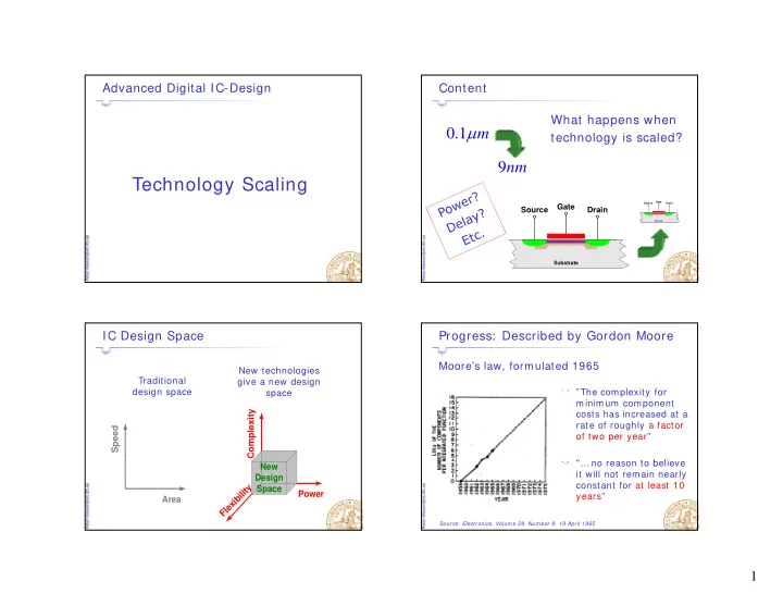
Full (ideal) Transistor Scaling

Original device

VD t

Scaled device (New Technology)

VD/S

t /S

Drain Gate Source

tox L

Channel length (L) Channel width (W)

ID

Drain Gate Source

tox/S

L/S

Channel length (L/S) Channel width (W/S)

ID/S Increased acceptor concentration for constant electrical field

Channel width (W) Thin oxide thickness (tox) Drain current (ID) Voltage (VD, VT, VDD, etc.) Doping (NA) Channel width (W/S) Thin oxide thickness (tox/S) Drain current (ID/S) Voltage (VD/S, VT/S, VDD/S, etc.) Doping (SNA)

Scaling Factors: Area & Capacitance

• x
• x
• x

W L W L C W L t ε ∝ × ∝ × × = × × Area Capacitance

2 2 2

1 / 1

• x
• x
• x

S S W L WL WL S S S C S t S ε ∝ × ⇒ = ∝ × = × ⇒ = Area Scaling factor Capacitance Scaling factor

tox L W

• x

ε = Material constant

Scaling Factor: Delay V

2 2

( ) ( ) ( )

L DD L OH OL n GS n DD T pHL H T L p

Q C V C V V Q I t k V V t C V k V V t = × Δ = − = = × = − × = × −

CL

2

( )

L n D pH DD L D T

C V k V t V − =

SLIDE 11

11

Scaling Factor: Delay (tp)

• x

W k C L μ μ = = = Gain factor Electron mobility

2 2 2 2 2

( ) ( ) ( )

• x

DD L DD DD p DD T DD T

• x

DD T DD

C WL V C V L V t W k V V V V C V V L V L μ μ × × ∝ ∝ ∝ − − −

2 2 2

( ) 1

DD p DD T

S S S S t V V μ ∝ ⇒ = − Scaled delay Scalning factor

Source: J. Rabaey, Digital Integrated Circuits

tox L W 2 2 L DD L DD p

C V P C V f t = ∝

Scaling Factor: Power Consumption

• x

t ε = = Material constant Delay

• x

L

• x
• x

C W LC WL t ε ε = =

tox L W

p

t Delay

2 2

• x

DD

• x

L DD p

WL V t P C V f t ε = ∝

Source: J. Rabaey, Digital Integrated Circuits

Delay (factor 1/S)

2 2

P

• x

DD

• x

L DD p

WL V t C V f t ε = ∝

Scaling Factor: Power Consumption

2 2 2 p

• x

DD

• x

p

V WL t t S S S S ε ∝ ⇒ Scaled power

2

1 S ⇒ = Scaling factor

2

1 S ⇒ = Power consumption Scaling factor

Scaling Factor: Power Consumption

2

1 S S ⇒ = Area Scaling factor Power consumption 1 ⇒ = Power consumption Scaling factor Area unit

SLIDE 12

12

Ideal Scaling: Limitation

Voltage scale less than other parameters d h h f ld h h l Leads to higher E-field in the channel Leads to saturation of the electron velocity Electron velocity

e- e- e- e- e-

Electron velocity cannot have an unlimited increase

High E-field

Velocity Saturation

´ ( )2

n

k W I V V =

N t t d

( ) 2

D GS T

I V V L = −

Non-saturated

´ ( ) 2

n D GS T

k W I V V L α = −

Velocity Saturated

2 α <

The drain current is reduced due to the velocity saturation

2 L

Saturated Velocity Saturation (0.25um technology)

α

2.1

Low VDD: Velocity Saturation can be neglected

1.7 1.8 1.9 2.0

High VDD: α decreases Saturation appear earlier in denser technologies

´ k W α

2.0 1.0 3.0 1.5 2.5 1.5 1.6

VDS [V]

Source: M. R. Stan, IEEE Trans. on VLSI Systems, Apr 01.

( ) 2

n D GS T

k W I V V L α = −

Velocity Saturation

VGS=5V

Short Long

VGS=3V VGS=4V VGS=2V

ID

Linear Dependence V Id V Id Short Device Long Device

1 2 3 4 5 VDS [V] VGS=1V

VGS

(Saturated Region)

VGS

SLIDE 13

13

Delay

2 2 2 2

( ) 1

DD DD T

S S S V L V V ∝ ⇒ = − Non- saturated gate delay Scaling factor

2 2 2 2 2 2

( ) 1

DD DD T

S S S L V V V L ∝ ⇒ = − Fixed voltage gate delay Scaling factor

2 2

1 (or ) (

DD DD T

S S L V V V α ∝ ⇒ −

<

Saturated gate delay Scaling factor 1) S The current do not increase as ”expected” at high voltages

Power

2 2 2 2

1

• x

DD

• x

V WL t t S S S S ε ∝ ⇒ = Non- saturated power consumption Scaling factor

2 2 2 2 2 2 pHL

• x

DD

• x

pHL

• x

DD

• x

t WL V t t WL V t S S S S S S S S ε ε ∝ ⇒ = Fixed- voltage power consumption Scaling factor Saturated power consumption ( 1) S ⇒

<

Scaling factor

The current do not increase as ”expected” at high voltages

• x

∝ Saturated power consumption (or 1)

pHL

S S t ⇒

<

Scaling factor

Transistor Scaling

Parameter Full Scaling Fixed Voltage Saturated Scaling g Voltage Scaling

Dimensions (W, L, and t ox) 1/ S 1/ S 1/ S VDD and VT0 1/ S 1 1 Delay 1/ S 1/ S2 1/ S Capacitance 1/ S 1/ S 1/ S I D 1/ S S 1 Power consumption 1/ S2 S 1 Power per area unit 1 S3 S2

We will compare to ITRS later Voltage do not scale: leads to increased power consumption

Dynamic Power Consumption

Partly limited by velocity saturation Dependent on technology type

2 L DD

P C V f =

Dependent on technology type

Technologies for high performance: Increased consumption Technologies for low power: Low voltage, less increase in power consumption

SLIDE 14

14

Power in new technologies?

Dynamic power have been dominating Static power will increase drasticaly How about interconnections? How about interconnections?

Metal Layers

Year 2001 2003 2005 2007 2010 2016 Techology (nm) 150 107 80 65 45 22 Metal Layers 7 8 9 9 10 10

Metal Layers - Not a 2D problem!!!

Transistors Transistors Tungsten Contacts

Delay vs Technology

Delay [ ps]

30 35 40

Interconnect Delay

5 10 15 20 25

Gate Delay

Source: SIA Roadmap

Technology [ um] 1989 1992 1995 1998 2001 2004 2007

0.65 0.5 0.35 0.25 0.18 0.13 0.1

SLIDE 15

15

Capacitive load will increase

Contacts

Plate Plate capacitors was dominating Fringing capacitors will

Fringing Capacitors

will dominate in new technologies

Interconnections on a Silicon Die

0.08 Connection Probability

Local Wires Global Wires

0.06 0.04

Global Wires

0.02 1.0 0.2 0.8 0.6 0.4 Wire Length/Chip Diagonal Length

do not scale with the technology

Comparison of Network-on-Chip and Busses

Copper Wires

40 % reduction in resistance 12 % performance improvement in a Power PC p p Transistor

SLIDE 16

16

Delay vs. Technology

Interconnect dominates the load

• Fringing capacitances added

3 dimensions

• 3 dimensions
• “Longer” global wires

Solutions?

• Copper wires
• Materials with low dielectric constant

Materials with low dielectric constant

• Interconnect optimization methodology

Physical design must be considered in all design phases

High performance:

Total power per function

Trends for Maximum Power

P [ W]

300 Low power: Doubling

• ver 15 years

High performance: Doubling over 15 years Idag, 150W 2016, 290W 300 100 200 158W Today,

Source: ITRS 2002 Update

Standby: Constant over 15 years

2001 2003 2005 2007 2010 2016 2013

100 3W

What about Moore’s Law?

The number of transistors is doubled every 18th month (1965) Gordon Moore

25

Moore’s lag: Total power?

100 W today 25 kW the year 2020

10 15 20 25

P (kW)

25 kW per chip!!!

2008 2010 2012 2014 2016 2018 2020 5

P År

Year

SLIDE 17

17

Manufacturing Costs

Initial cost have the largest increase Smaller sizes leads to an explosion of the

2 Mask set cost [M$] 1

costs for a mask-set

2M$

0.80 0.07 0.10 0.13 0.15 0.18 0.25 0.35 0.60 Feature size 1

Source: eASIC

Source: eASIC

Manufacturing Costs - Masks

2500

Cost ($1000)

1000 2000

45 nm 65 nm 90 nm

More Expensive in the beginning Exponential cost increase 2008 1995 2002

Year

130 nm 180 nm 250 nm Source: Jan Rabaey

Manufacturing costs in new Technologies

More Expensive for lower volumes but cheaper when the volumes goes up

130 nm t / Die ($) 180 nm Volume (Dies) Cost

Cost per Function (CPF)

CPF reduction between 29-35% per year

Technology 1

cost per function

0.1 1 Technology cross over Technology 1 Technology 2 Technology 3

Source: Rakesh Kumar

Relative Years

0.01

2 4 6 8 10 12

Technology cross-over

SLIDE 18

18

Costs – New Fab

Capital Cost (M$)

3000 12"

2.5 Billion $

2000 1000 6" 8"

$ Technology

0.8 2 0.5 0.25 0.15 0.13 0.8 0.07 5" 6"

What is volume?

Typical "business case" for an ASIC (130 nm): Price of "off-the-shelf" IC - 50$ per Chip Price of off the shelf IC 50$ per Chip Manufacture cost - 10$ per Chip Development costs - 20M$

50$ 10$ Break-even 500000 Chips − =

Source: Peter Olanders, Ericsson

Break even 500000 Chips 20M$

Break-even is higher for 90 nm, 65nm …

Increase from 50% to over 90% of the silicon area

Memories on Chip

20% 40% 60% 80% 100% % Area Memory % Area Reused Logic 0% 20% 1 9 9 9 2 2 2 5 2 8 2 1 1 2 1 4 g % Area New Logic

source: Japanese system-LSI industry