SVM vs Regularized Least Squares Classification Peng Zhang and Jing - PDF document

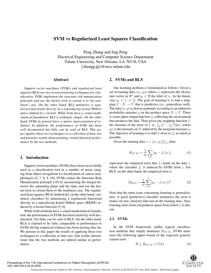
SVM vs Regularized Least Squares Classification Peng Zhang and Jing Peng Electrical Engineering and Computer Science Department Tulane University, New Orleans, LA 70118, USA { zhangp,jp } @eecs.tulane.edu Abstract 2. SVMs and RLS Our learning problem is formulated as follows: Given a Support vector machines (SVMs) and regularized least set of training data: ( x i , y i ), where x i represents the i th fea- squares (RLS) are two recent promising techniques for clas- ture vector in ℜ n and y i ∈ ℜ the label of x i . In the binary sification. SVMs implement the structure risk minimization case y i ∈ {− 1 , 1 } . The goal of learning is to find a map- principle and use the kernel trick to extend it to the non- ping f : X → Y that is predictive (i.e., generalizes well). linear case. On the other hand, RLS minimizes a regu- The data ( x, y ) is drawn randomly according to an unknown larized functional directly in a reproducing kernel Hilbert probability measure ρ on the product space X × Y . There space defined by a kernel. While both have a sound math- is a true input-output function f ρ reflecting the environment ematical foundation, RLS is strikingly simple. On the other that produces the data. Then given any mapping function f , hand, SVMs in general have a sparse representation of so- X ( f − f ρ ) 2 dρx , where � the measure of the error of f is: lutions. In addition, the performance of SVMs has been ρx is the measure on X induced by the marginal measure ρ . well documented but little can be said of RLS. This pa- The objective of learning is to find f close to f ρ as much as per applies these two techniques to a collection of data sets possible. and presents results demonstrating virtual identical perfor- Given the training data z = { x i , y i } m mance by the two methods. i =1 , then l R SV M = 1 � | y i − f z ( x i ) | (1) m 1. Introduction i =1 represents the empirical error that f z made on the data z , Support vector machines (SVMs) have been successfully where the classifier f z is induced by SVMs from z . For used as a classification tool in a number of areas, rang- RLS, on the other hand, the empirical error is ing from object recognition to classification of cancer mor- phologies [4, 7, 8, 9, 10]. SVMs realize the Structure Risk l R RLS = 1 � ( y i − f z ( x i )) 2 . Minimization principle [10] by maximizing the margin be- (2) m tween the separating plane and the data, and use the ker- i =1 nel trick to extend them to the nonlinear case. The regular- Note that the main issue concerning learning is generaliza- ized least squares (RLS) method [6], on the other hand, con- tion. A good (predictive) classifier minimizes the error it structs classifiers by minimizing a regularized functional makes on new (unseen) data not on the training data. Also, directly in a reproducing kernel Hilbert space (RKHS) in- learning starts from a hypothesis space from which f is cho- duced by a kernel function [5, 6]. sen. While both methods have a sound mathematical founda- tion, the performance of SVMs has been relatively well doc- 2.1. SVMs umented. Yet little can be said of RLS. On the other hand, RLS is claimed to be fully comparable in performance to In the SVM framework, unlike typical classifica- SVMs [6] but empirical evidence has been lacking thus far. tion methods that simply minimize R SV M , SVMs mini- We present in this paper the results of applying these two mize the following upper bound of the expected general- techniques to a collection of data sets. Our results demon- ization error strate that the two methods are indeed similar in perfor- R ≤ R SV M + C ( h ) , mance. (3) Proceedings of the 17th International Conference on Pattern Recognition (ICPR’04) 1051-4651/04 $ 20.00 IEEE Authorized licensed use limited to: MIT Libraries. Downloaded on February 16,2010 at 20:28:22 EST from IEEE Xplore. Restrictions apply.

where C represents the “VC confidence,” and h the VC di- K where is the Gram (kernel) matrix, and ( y 1 , y 2 , · · · , y m ) t . The resulting classifier f is y = mension. This can be accomplished by maximizing the mar- (in the appendix, we show how to derive f ) gin between the separating plane and the data, which can be viewed as realizing the Structure Risk Minimization princi- � f ( x ) = c i K ( x, x i ) (9) ple [10]. The SVM solution produces a hyperplane having the For the binary classification { -1,1 } case, if f ( x ) ≤ 0 , the maximum margin, where the margin is defined as 2 / � w � . predicted class is − 1 . Otherwise it is 1 . Note that there is no It is shown [1, 4, 10] that this hyperplane is optimum with issue of separability or nonseparability for this algorithm. respect to the maximum margin. The hyperplane, deter- mined by its normal vector � w � , can be explicitly written as w = � i ∈ SV α i y i x i , where α i ’s are Langrange coeffi- 2.3. Complexity cients that maximize The bulk of the computational cost associated with α i − 1 � � L D = α i α j y i y j x i · x j (4) SVMs is incurred by solving the quadratic program- 2 i i,j ming problem (4). This optimization problem can be bounded by O ( N 3 s + N 2 s m + N s nm ) [1], where N s is the and SV is the set of support vectors determined by the number of support vectors and n the dimensions of the in- SVM. For the nonlinear case, the dot product can be re- put data. In the worst case, N s ≈ m , we have O ( nm 2 ) . placed by kernel functions. On the other hand, solving the linear system of equa- tions (8) has been studied for a long time, and efficient al- 2.2. RLS gorithms exist in numerical analysis (the condition number is good if mγ is large). In the worst case, it can be bounded Starting from the training data z = ( x i , y i ) m and the i by O ( m 2 . 376 ) [3]. Overall, a RLS solution can be obtained unknown true function f ρ , instead of looking for the the much faster than that computed by SVMs. However, a SVM � l 1 empirical optimal classifier that minimizes i =1 ( y i − m solution has a sparse representation, which can be advanta- f z ( x i )) 2 , RLS focuses on the problem of estimating [5, 6] geous in prediction. � ( f z − f ρ ) 2 dρ X . (5) 3. Experiments X In order to search f z , it begins with a hypothesis space H . The RLS algorithm can be implemented in a straight for- Define the “true optimum” f H relative to H . That is, f H = ward way. For SVMs, we used the package from LIBSVM X ( f − f ρ ) 2 dρ X . � min [2]. For both algorithms we adopt the same kernel function: H Gaussian K ( x, x ′ ) = e −� x − x ′ � 2 / 2 σ 2 . The problem above can then be decomposed as [6]: The SVM algorithm has two procedural parameters: σ � � ( f z − f ρ ) 2 dρ X = S ( z, H ) + ( f H − f ρ ) 2 dρ X and C , the soft margin parameter. Similarly, the RLS algo- (6) X X rithm also has two parameters: σ and γ . σ is common to both. For model selection, ten-fold cross-validation is used. X ( f z − f ρ ) 2 dρ X − � X ( f H − f ρ ) 2 dρ X . where S ( z, H ) = � σ takes values in [ 10 − 15 , 10 15 ], C in [ 10 − 15 , 10 15 ], and γ On the right-hand side of (6), the first term is called sample in [ 10 − 15 , 10 5 ]. error or sometime estimation error, while the second term is called approximation error [6]. 3.1. Real Data Experiments The RLS algorithm chooses RKHS as the hypothesis space H K , and minimizes the following regularized func- 12 datasets from UCI Machine Learning Reposi- tional: 1 ( y i − f ( x i )) 2 + γ � f � 2 tory were used for comparison. They are: glass, cancer, � (7) K m cancer-w, credit card, heart cleveland, heart hungery, iono- sphere, iris, letter (only v and w are chosen), new thyoid, where � f � 2 K is the norm in H K defined by the kernel K , pima indian, and sonar. Some datasets has minor miss- and γ a fixed parameter. The minimizer exists and is unique ing data. In that case, the missing data are removed. All [6]. features are normalized to lie between 0 and 1. For ev- It turns out that the solution to the above optimization problem is quite simple: Compute c = ( c 1 , c 2 , · · · , c m ) t by ery dataset, we randomly choose 60% as training data and the rest 40% as testing data. The process is re- solving the equation peated 10 time and the average error rates obtained by the ( mγI + K ) c = y (8) two methods are reported. Proceedings of the 17th International Conference on Pattern Recognition (ICPR’04) 1051-4651/04 $ 20.00 IEEE Authorized licensed use limited to: MIT Libraries. Downloaded on February 16,2010 at 20:28:22 EST from IEEE Xplore. Restrictions apply.