survey sampling Risto Lehtonen University of Helsinki BaNoCoSS - PowerPoint PPT Presentation
On balanced sampling and calibration estimation in survey sampling Risto Lehtonen University of Helsinki BaNoCoSS 2019, rebro University, 16-20 June 2019 Topics to be addressed Motivation Representative strategy by Hjek Balanced sampling
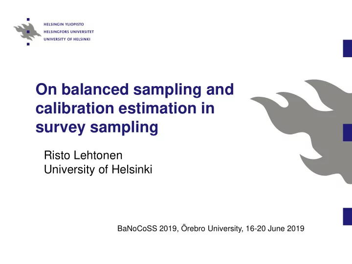
On balanced sampling and calibration estimation in survey sampling Risto Lehtonen University of Helsinki BaNoCoSS 2019, Örebro University, 16-20 June 2019
Topics to be addressed Motivation Representative strategy by Hájek Balanced sampling & calibration estimation Hájek and HT type calibration estimators Examples Discussion 2
Jaroslav Hájek (1926-1974) Important contributions in statistics: Representative strategy à la Hájek Hájek J. (1959) Optimum strategy and other problems in probability sampling, Casopis pro Pestováni Matematiky, 84, 387 – 423. Hájek estimator of population mean under unequal probability sampling Hájek J. (1971) Comment on “An essay on the logical foundations of survey sampling” by Basu, D. In Godambe V.P. and Sprott D.A. (eds.) Foundations of Statistical Inference, p. 236. Holt, Rinehart and Winston. 3
Motivation METRON - International Journal of Statistics 2011, vol. LXIX, n. 1, pp. 45-65 MATTI LANGEL – YVES TILLÉ 4
Representative strategy in the spirit of Jaroslav Hájek (1959, 1981) Strategy : a couple of sampling design and estimation design Representative strategy : strategy that estimates the totals of auxiliary variables exactly (without error) Let ( , ,..., ) be our auxiliary data vector for unit z z z z k U 1 2 k k k Lk in population {1 ,..., ,..., } U k N Define weights for such that w k U k the representativeness equations w z z k k k k s k U are fulfil led, where denotes a sample from s U 5
Options It is obvious that a representative strategy can be constructed under the sampling design o under the estimation design o o under both the sampling and estimation designs For sampling design, ( , ,..., ) denotes the auxiliary z z z z 1 2 k k k Lk data vector for unit in population {1 ,..., ,..., } k U k N For estimation design, let ( , ,..., ) be another x x x x 1 2 k k k Jk auxiliary data vecto r for unit in k U z-vectors and x-vectors may be separate or overlapping vectors 6
Strategy 1: Horvitz-Thompson estimation for a balanced probability sample Representativeness through the sam pling design Auxiliary data are incorporated in the sampling procedure Deville and Tillé 2004 , T illé 2 11 0 Compute i nclusion probabilities that satis f y Sampling design : k the for any sample : balancing equations s / z z k k k k s k U Horvitz-Thompson estimator Estimation design: ˆ t a y HT k k k s where 1/ are design weights a k k The sampling design is balanced on the a uxiliary z-variables 7
Strategy 2: Calibration estimation for a (generic) probability sample Representativeness through the estimation design Auxiliary data are incorporated in the estimation procedure Deville & Särndal 1992 , Särndal (2007) Compute adjustment factors that satisfy g k th e for the given probability sample calibr ation equations s / g x x k k k k k s k U : Model-free calibration estimator Estimation design ˆ t w y CAL k k k s where / are calibration weights w g k k k The estimation desi gn is balanced on the auxiliary x-variables 8
Remarks In practical applications, the availability & share of labour between the auxiliary z-data (sampling phase) and auxiliary x-data (estimation phase) becomes an issue Balanced sampling: z-data are needed at the sampling unit level Calibration estimation: x-data are needed either at an aggregate level or at the unit level, depending on the calibration method 9
Basic developments Sampling design: The CUBE method Deville and Tillé (2004) Efficient balanced sampling: The cube method (Biometrika). Penalization: Breidt and Chauvet (2012) Penalized balanced sampling (Biometrika). Estimation design: Calibration Deville and Särndal (1992). Calibration estimators in survey sampling (JASA). Penalization: Guggemos and Tillé (2010) Penalized calibration in survey sampling: Design-based estimation assisted by mixed models (Journal of Statistical Planning and Inference). 10
11
Example 1: Deville & Tillé (2004) {1 ,..., ,..., } real population (MU284), 280 U k N N ( , , , ) , auxiliary data vector z z z z z k U 1 2 3 4 k k k k k for both sample balancing and calibration estimation 1/ design weights a k k calibration weights w g a k k k ˆ HT estimators of totals of : ( ) , 1 ,...,6 y t y a y j j HT j k jk k s ˆ ˆ ˆ Calibration estimators ( ) ( ) ( ) t y w y t y t t B CAL j k jk HT j z HTz j k s 1 where B a z z a z y j k k k k k jk k s k s Simulation exp er iments 1000 fi xed-size samples from , 20 K U n 12
...contd. Strategies for the 6 target variables y , ,..., y y 1 2 6 a Non-balanced sampling and HT estimation ) b Balanced sampling and HT ) c Non-balanced sampling and CAL estimation ) d Balanced sampling and ) CAL NOTE: Act ually, sampling in a) and c) is with balancing with CUBE but on a single variable ( ) z 1 13
Results on accuracy Table1 Estimators of population total: Monte Carlo MSE relative to the MSE for non-balanced sampling with HT estimator Horvitz-Thompson Calibration Target Non- Non- Balanced Balanced variable balanced balanced samples samples samples samples y 1 0.90 0.82 0.76 1 y 1 0.91 1.02 0.87 2 y 1 0.80 0.92 0.82 3 y 1 0.21 0.11 0.11 4 y 1 0.15 0.21 0.08 5 y 1 0.26 0.15 0.14 6 Extracted from Deville & Tillé (2004) p. 909 Table 1 14
Analysis Table 2 Correlation of auxiliary Target Balancing Balancing variables with target variables variable y & HT & CAL in the population and R square y 0.90 0.76 for regression model ( N =280) 1 y 0.91 0.87 2 Target variables Auxiliary y 0.80 0.82 3 variables y y y y y y 1 2 3 4 5 6 y 0.21 0.11 4 - 0.99 0.63 0.87 0.89 - z 1 y 0.15 0.08 5 - 0.99 0.65 0.85 0.90 - z y 2 0.26 0.14 6 - - - - - - z 3 Correlation of aux. var. z - 0.99 0.64 0.85 0.90 - z 4 z z z z 1 2 3 4 - 0.99 0.42 0.76 0.81 - 2 R z 1.00 0.99 - 0.98 1 - no data z 0.99 1.00 - 0.99 2 z 1.00 - - - 3 z 0.98 0.99 1.00 4 15
COMMENT: Interesting empirical exploration on the interplay between balanced sampling and calibration estimation by simulation experiments using real survey data Several strategies are applied by combining balanced and non-balanced sampling and Horvitz-Thompson and calibration estimators www.statisticsjournal.lt 16
Remarks The previous representative design-based strategies were model-free because statistical models did not play an explicit role Model-assisted methods in representative design-based strategies: o Balanced sampling Penalized balanced sampling (Breidt & Chauvet 2012) o Calibration estimation Penalized calibration (Guggemos & Tillé 2010) Generalized calibration (Deville 2000) Model calibration (Wu & Sitter 2001) o Calibration in small domain estimation Model-assisted calibration (Lehtonen & Veijanen 2012, 2016) Multiple model calibration (Montanari & Ranalli 2009) Two-level hybrid calibration (Lehtonen & Veijanen 2017) 17
18
Example 2: Breidt & Chauvet (2012) Linear mixed modeling in penalized balanced sampling by relaxing some balance constraints Analogous to the use of penalization at the estimation stage (Guggemos & Tillé 2010) for reducing some calibration constraints Why? Ordinary balanced samples may reduce the need for calibration weighting in the estimation phase (Deville & Tillé example) Penalized balanced samples may reduce the need for linear mixed modeling (penalized calibration) in the estimation phase Gain: HT estimators for penalized balanced samples will be efficient for target variables well approximated by a linear mixed model , x β z u y k U k k k k where are fixed effects and are random effects β u 19
Breidt & Chauvet contd. Monte Carlo study i ncluding balanced sampling guided by a penalized spline expressed as a linear mixed model Generated artificial population of 1 000 N 1 Auxiliary variable (1 ) , lognormal x z z 1 1 1 k k 1 (1 ) , lognormal, independent of x z z z 2 2 2 1 k k Target variables y and y 1 2 Linear model 1 2( 0.5), Exponent ial mode l e xp( 8 ) m x m x 2 6 Sampling designs defined by x 1 Estimatio n designs for y defined b y x and for y by x 1 1 2 2 Strategy (x : x ) x for sampling design & estimation design 1 1 1 Strategy (x : x ) x for sampling design and x for estimation design 1 2 1 2 Simulation experiments: 5000 simulated sample s of size 100 K n 20
Recommend
More recommend
Explore More Topics
Stay informed with curated content and fresh updates.




![CS786 Lecture 13: May 14, 2012 Sampling techniques [KF Chapter 12] CS786 P. Poupart 2012 1](https://c.sambuz.com/696755/cs786-lecture-13-may-14-2012-s.webp)
