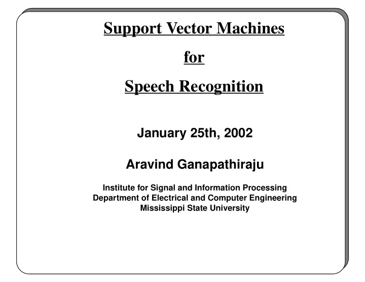
Support Vector Machines for Speech Recognition January 25th, 2002 - PowerPoint PPT Presentation
Support Vector Machines for Speech Recognition January 25th, 2002 Aravind Ganapathiraju Institute for Signal and Information Processing Department of Electrical and Computer Engineering Mississippi State University Organization of
Support Vector Machines for Speech Recognition January 25th, 2002 Aravind Ganapathiraju Institute for Signal and Information Processing Department of Electrical and Computer Engineering Mississippi State University
Organization of Presentation * Motivation for using support vector machines (SVM) * SVM theory and implementation * Issues in using SVMs for speech recognition — hybrid recognition framework * Experiments — data description and experimental results * Error analysis and oracle experiments * Summary and conclusions including dissertation contributions
Motivation * Need discriminative techniques to enhance acoustic modeling * Maximum Likelihood-based systems can be improved upon by discriminative machine learning techniques * Support Vector Machines (SVM) have had significant success on several classification tasks * Efficient estimation techniques now available for SVMs * Study the feasibility of using SVMs as part of a full- fledged conversational speech recognition system
ASR Components Input Speech Acoustic Front-End Focus of Statistical Acoustic Dissertation Models p(A/W) Language Search Model p(W) Recognized Utterance * Dissertation addresses acoustic modeling
Acoustic Modeling a 11 a 22 a 55 a 33 a 44 1 2 3 4 5 a 13 a 35 a 24 ( ) ( ) ( ) ( ) ( ) b 1 o t b 2 o t b 5 o t b 3 o t b 4 o t * HMMs used is most state-of-the-art systems * Maximum likelihood (ML) estimation dominant approach * Expectation-maximization algorithm * Hybrid Connectionist Systems — artificial neural networks (ANNs) used as probability estimators
SVM Success Stories * SVMs have been used in several static classification tasks since the 1990’s * State-of-the-art performance on the NIST handwritten digit recognition task (Vapnik et al.) — 0.8% error * State-of-the-art performance on Reuters text categorization (Joachims et al.) — 13.6% error * Faster training/estimation procedures allow for use of SVMs on complex tasks (Osuna et al.) * Significant SVM research advances beyond classification — transduction, regression and function estimation
Representation Vs. Discrimination 0.03 0.4 0.025 Optimal 0.02 Decision Boundary 0.3 0.015 0.01 0.2 0.005 ML Decision Boundary 0 4 3.5 4.5 5 0.1 0 0 10 20 30 40 * Efficient estimation procedures for classifiers based on ML — expectation-maximization makes ML feasible for complex tasks * Convergence in ML does not necessarily translate to optimal classification
Risk Minimization * Risk minimization often used in machine learning R α ( ) Q z α ( , ) d P z ( ) , α ∈ Λ ∫ = α : defines the parametrization : is the loss function Q : belongs to the union of the input and output spaces z : describes the distribution of . P z * Loss functions can take several forms (squared error) * Avoid estimation of by using empirical risk P 1 Remp α ( ) ∑ Q zi α ( , ) , α ∈ Λ = - - - l * Minimum empirical risk can be obtained by several configurations of the system
Structural Risk Minimization bound on the expected risk expected risk optimum confidence in the risk empirical risk VC dimension * Control over generalization R α ( ) ≤ Remp α ( ) ( ) + f h * , the VC Dimension is a measure of the capacity of the h learning machine
Optimal Hyperplane Classifiers C2 H2 CO C1 class 1 H1 w origin optimal classifier class 2 * Hyperplanes C0, C1 and C2 achieve perfect classification — zero empirical risk * However, C0 is optimal in terms of generalization
Optimization ⋅ * Hyperplane: x w + b ( ⋅ ) ≥ ∀ * Constraints: yi x i w + b – 1 0 i N N 2 1 ∑ ∑ α iyi x i w ( ⋅ ) α i * Optimize: - - w - LP = – + b + 2 i = 1 i = 1 * Lagrange functional setup to maximize margin while satisfying minimum risk criterion numSVs ∑ ( ) α iyi x i x ⋅ * Final classifier: f x = + b i = 1
Soft Margin Classifiers + training error for class 1 + training error for class 2 * class 1 class 2 w H2 * - b/| w | H1 origin * Constraints modified to allow for training errors ( ⋅ ) ≥ ξ i ∀ yi x i w + b 1 – i * Error control parameter, used to penalize training C errors
Non-linear Hyperplane Classifiers * Data for practical applications typically not separable using a hyperplane in the original input feature space * Transform data to higher dimension where hyperplane classifier is sufficient to model decision surface Φ : ℜ n ℜ N → * Kernels used for this transformation ( , ) Φ xi ( ) Φ x j ⋅ ( ) K xi x j = numSVs ∑ ( ) α iyiK x xi ( , ) * Final classifier: f x = + b i = 1
Example Non-Linear Classifier 2-dimensional input space class 1 * * + class 2 decision boundary class 1 data points: (-1,0) (0,1) (0,-1) (1,0) class 2 data points: 3-dimensional transformed space (-3,0) (0,3) (0,-3) (3,0) class 1 data points: (1,0,0) (0,1,0) (0,1,0) (1,0,0) class 2 data points: x 2 y 2 ( , ) ⇒ ( , , ) (9,0,0) (0,9,0) (0,9,0) (9,0,0) x y 2 xy
Practical SVM Training Working Set Defn. Optimize Working Set Optimize Working Set training steepest feasible direction data quadratic optimization quadratic optimization Terminate? Terminate? yes yes no check for change in check for change in SVM multipliers multipliers * “Chunking” — proposed by Osuna et al. * Guarantees convergence to global optimum * Working set definition is crucial
From Classifiers to Recognition * ISIP ASR system used as the starting point ( ⁄ ) * Likelihood-based decoding — used log P A M * SVMs do not generate likelihoods ( ⁄ ) P A ( ) P M A ( ⁄ ) P A M = - - - - - - - - - - - - - - - - - - - - - - - - - - - - - - - - - - - - ( ) P M ( ) ( ) * Ignore and use model priors P A P M * Posterior estimation required * Feature space needs to be decided — frame level data vs. segment level data * Use SVM derived posteriors to rescore N-best lists
Posterior Estimation negative examples positive examples probability 1 ( ⁄ ) p y f = 1 = - - - - - - - - - - - - - - - - - - - - - - - - - - - - - - - - - - - - - - - - - - ( ) 1 + exp Af + B SVM Distances * Gaussian assumption is good for overlap region * Leads to compact distance-posterior transformation — sigmoid function
Segmental Modeling k frames hh aw aa r y uw region 1 region 2 region 3 0.3*k frames 0.4*k frames 0.3*k frames mean region 1 mean region 2 mean region 3 * Allows for each classifier to be exposed to a limited amount of data. * Captures wider contextual variation * Approach successfully used in segmental ASR systems where Gaussians are used to model segment duration
Hybrid Recognition Framework HMM mel-cepstral data recognition segment information convert to segmental data N-best information segmental features hybrid decoder hypothesis * Gaussian computations replaced with SVM-based probabilities in the hybrid decoder * Composite feature vectors generated based on traditional HMM-based alignments
Processing Alternatives * Basic hybrid system operates on a single hypothesis- derived segmentation * Approach is simple and saves computations * Alternate approach involves N segmentations * Each segmentation derived from the corresponding hypothesis in the N-best list * Computationally expensive * Closer in principle to other rescoring-based hybrid frameworks * Allows for SVM and HMM score combination
Experimental Data - Deterding Vowel * Often used for benchmarking non-linear classifiers * 11 vowels spoken in a “h*d” context * Training set consists of 528 frames of data from 8 speakers * Test set composed of 476 frames from seven speakers * Small size of training set makes the dataset challenging * Best result reported on this dataset — 29.6% error
Results - Static Data Classification gamma classification error C classification error (C=10) % (gamma=0.5) % 0.2 45 1 58 0.3 40 2 43 0.4 35 3 43 0.5 36 4 43 0.6 35 5 39 0.7 35 8 37 0.8 36 10 37 0.9 36 20 36 1.0 37 50 36 100 36 * Best SVM performance: 35% classification error with RBF kernels * Polynomial kernels perform worse — best performance was a 49% classification error
Experimental Data - OGI Alphadigits * Telephone database of 6-word strings * Training Data * 52000 sentences * 1000 sentences as cross-validation set to estimate sigmoid parameters * Test data * 3329 sentences — speaker independent open-loop test set * Number of phone classifiers — 30 * 39-dimensional MFCC features used
OGI Alphadigits (AD): Effect of Segment Proportion Segmentation WER (%) WER (%) Proportions RBF kernel polynomial kernel 2-4-2 11.0 11.3 3-4-3 11.0 11.5 4-4-4 11.1 11.4 * Previous research suggests 3-4-3 proportion (Glass, et al.) * For SVM classifiers, segment proportion does not have any significant impact on classifier accuracy or system performance, especially with RBF kernels * 3-4-3 proportion used for all further experiments
Recommend
More recommend
Explore More Topics
Stay informed with curated content and fresh updates.
