Supervised Learning II Cameron Allen csal@brown.edu Fall 2019 - PowerPoint PPT Presentation
Supervised Learning II Cameron Allen csal@brown.edu Fall 2019 Machine Learning Subfield of AI concerned with learning from data . Broadly, using: Experience To Improve Performance On Some Task (Tom Mitchell, 1997) Supervised
Supervised Learning II Cameron Allen csal@brown.edu Fall 2019
Machine Learning Subfield of AI concerned with learning from data . Broadly, using: • Experience • To Improve Performance • On Some Task (Tom Mitchell, 1997)
Supervised Learning Input: inputs X = {x 1 , …, x n } training data Y = {y 1 , …, y n } labels Learn to predict new labels . Given x: y?
Supervised Learning Input: inputs X = {x 1 , …, x n } training data Y = {y 1 , …, y n } labels Learn to predict new labels . Given x: y? “Not Hotdog”, SeeFood Technologies Inc.
Supervised Learning Input: inputs X = {x 1 , …, x n } training data Y = {y 1 , …, y n } labels Learn to predict new labels . Given x: y?
Supervised Learning Formal definition: Given training data: inputs X = {x 1 , …, x n } Y = {y 1 , …, y n } labels Produce: Decision function f : X → Y That minimizes error: X err ( f ( x i ) , y i ) i
Neural Networks σ ( w · x + c ) logistic regression
Deep Neural Networks o 1 o 2 h n1 h n2 h n3 …. h 11 h 12 h 13 x 1 x 2
Nonparametric Methods Most ML methods are parametric: • Characterized by setting a few parameters. • y = f ( x, w ) Alternative approach: • Let the data speak for itself. • No finite-sized parameter vector. • Usually more interesting decision boundaries.
K-Nearest Neighbors Given training data: X = {x 1 , …, x n } Y = {y 1 , …, y n } Distance metric D(x i , x j ) For a new data point x new : find k nearest points in X (measured via D) set y new to the majority label
K-Nearest Neighbors + + + + - - - + - + + - ++ + - + - -
K-Nearest Neighbors Decision boundary … what if k=1? + + + + - - - + - + + - ++ + - + - -
K-Nearest Neighbors Properties: • No learning phase. • Must store all the data. • log(n) computation per sample - grows with data . Decision boundary: • any function, given enough data. Classic trade-off: memory and compute time for flexibility.
Applications • Fraud detection • Internet advertising • Friend or link prediction • Sentiment analysis • Face recognition • Spam filtering
Applications MNIST Data Set Training set: 60k digits Test set: 10k digits
Classification vs. Regression If the set of labels Y is discrete: • Classification • Minimize number of errors If Y is real-valued: • Regression • Minimize sum squared error Let’s look at regression.
Regression with Decision Trees Start with decision trees with real-valued inputs. a > 3.1 false true y=1 b < 0.6? false true y=2 y=1
Regression with Decision Trees … now real-valued outputs. a > 3.1 false true y=0.6 b < 0.6? false true y=0.3 y=1.1
Regression with Decision Trees Training procedure - fix a depth, k . If you have k=1, fit the average. If k > 1: Consider all variables to split on Find the one that minimizes SSE Recurse ( k-1 ) What happens if k = N ?
Regression with Decision Trees (via scikit-learn docs)
Linear Regression Alternatively, explicit equation for prediction. Recall the Perceptron. If x = [ x(1), … , x(n) ]: + • Create an n -d line + + - + • Slope for each x(i) - • Constant offset + - + f ( x ) = sign ( w · x + c ) - gradient offset
Linear Regression Directly represent f as a linear function: • f ( x, w ) = w · x + c What can be represented this way? y x 2 x 1
Linear Regression How to train? Given inputs: • x = [ x 1 , …, x n ] (each x i is a vector, first element = 1) • y = [ y 1 , …, y n ] (each y i is a real number) Define error function: Minimize summed squared error n X ( w · x i − y i ) 2 i =1
Linear Regression The usual story: • Set derivative of error function to zero. n d ( w · x i − y i ) 2 = 0 X dw n ! i =1 X x T A = i x i n X ( w · x i − y i ) x T 2 i = 0 i =1 matrix i =1 n ! n n X X x T x T i x i w = i y i X x T b = i y i i =1 i =1 i =1 vector w = A − 1 b
Polynomial Regression More powerful: • Polynomials in state variables. • 1st order: [1 , x, y, xy ] • 2nd order: [1 , x, y, xy, x 2 , y 2 , x 2 y, y 2 x, x 2 y 2 ] • y i = w · Φ ( x i ) What can be represented?
Polynomial Regression As before … n d X ( w · Φ ( x i ) − y i ) 2 dw i =1 n Φ T ( x i ) Φ ( x i ) X A = i =1 w = A − 1 b n Φ T ( x i ) y i X b = i =1
Polynomial Regression (wikipedia)
Overfitting
Overfitting
Ridge Regression A characteristic of overfitting: • Very large weights. Modify the objective function to discourage this: n ( w · x i − y i ) 2 + λ || w || X min i =1 error term regularization term � − 1 A T b A T A + Λ T Λ � w =
Neural Network Regression σ ( w · x + c ) classification
Neural Network Regression output layer o 1 o 2 hidden layer h 1 h 2 h 3 input layer x 1 x 2
Neural Network Regression σ ( w o 2 1 h 1 + w o 2 2 h 2 + w o 2 3 h 3 + w o 2 4 ) σ ( w o 1 1 h 1 + w o 1 2 h 2 + w o 1 3 h 3 + w o 1 4 ) value computed o 1 o 2 feed forward h 1 h 2 h 3 σ ( w h 2 1 x 1 + w h 2 2 x 2 + w h 2 σ ( w h 3 1 x 1 + w h 3 2 x 2 + w h 3 3 ) 3 ) value computed h 1 = σ ( w h 1 1 x 1 + w h 1 2 x 2 + w h 1 x 1 x 2 3 ) input layer x 1 , x 2 ∈ [0 , 1]
Neural Network Regression A neural network is just a parametrized function: y = f ( x, w ) How to train it? Write down an error function: ( y i − f ( x i , w )) 2 Minimize it! (w.r.t. w ) No closed form solution to gradient = 0. Hence, stochastic gradient descent: d •Compute dw ( y i − f ( x i , w )) 2 •Descend
Image Colorization (Zhang, Isola, Efros, 2016)
Nonparametric Regression Most ML methods are parametric: • Characterized by setting a few parameters. • y = f ( x, w ) Alternative approach: • Let the data speak for itself. • No finite-sized parameter vector. • Usually more interesting decision boundaries.
Nonparametric Regression What’s the regression equivalent of k -Nearest Neighbors? Given training data: X = {x 1 , …, x n } Y = {y 1 , …, y n } Distance metric D(x i , x j ) For a new data point x new : find k nearest points in X (measured via D) set y new to the (weighted by D) average y i labels
Nonparametric Regression As k increases, f gets smoother.
Gaussian Processes
Applications model and predict variations in pH, clay, and sand content in the topsoil (Gonzalez et al., 2007)
Recommend
More recommend
Explore More Topics
Stay informed with curated content and fresh updates.
