Learning frameworks Self-supervised learning: (Auto)encoder networks - PowerPoint PPT Presentation
Learning frameworks Self-supervised learning: (Auto)encoder networks Supervised learning Network must copy inputs to outputs through Assumes environment specifies correct output (targets) for each input a bottleneck (fewer hidden units)
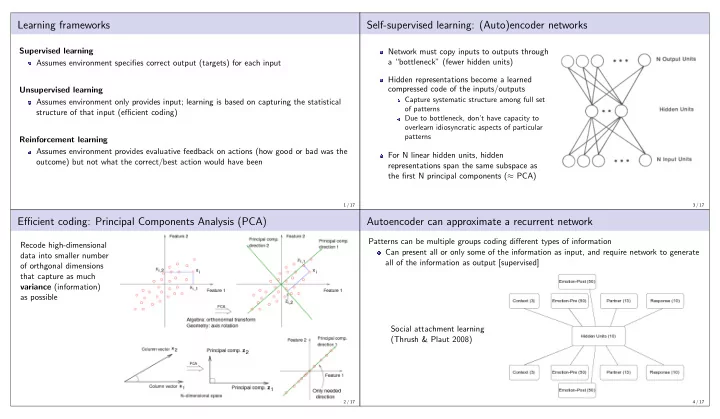
Learning frameworks Self-supervised learning: (Auto)encoder networks Supervised learning Network must copy inputs to outputs through Assumes environment specifies correct output (targets) for each input a “bottleneck” (fewer hidden units) Hidden representations become a learned compressed code of the inputs/outputs Unsupervised learning Capture systematic structure among full set Assumes environment only provides input; learning is based on capturing the statistical of patterns structure of that input (efficient coding) Due to bottleneck, don’t have capacity to overlearn idiosyncratic aspects of particular patterns Reinforcement learning Assumes environment provides evaluative feedback on actions (how good or bad was the For N linear hidden units, hidden outcome) but not what the correct/best action would have been representations span the same subspace as the first N principal components ( ≈ PCA) 1 / 17 3 / 17 Efficient coding: Principal Components Analysis (PCA) Autoencoder can approximate a recurrent network Patterns can be multiple groups coding different types of information Recode high-dimensional Can present all or only some of the information as input, and require network to generate data into smaller number all of the information as output [supervised] of orthgonal dimensions that capture as much variance (information) as possible Social attachment learning (Thrush & Plaut 2008) 2 / 17 4 / 17
Self-supervised learning: Prediction Restricted Boltzmann Machines Simple recurrent (sequential) networks Target output can be prediction of next input No connections among units within a layer; allows fast settling Fast/efficient learning procedure Can be stacked; successive hidden layers can be learned incrementally (starting closest to the input) (Hinton) 5 / 17 7 / 17 Boltzmann Machine learning: Unsupervised / generative version Hinton’s handwritten digit generator/recognizer Supervised version Negative phase : Clamp inputs only; run hidden and outputs units [cf. forward pass] Positive phase : Clamp both inputs and outputs (targets); run hidden [cf. backward pass] Unsupervised / generative version Positive phase : Visible units clamped to external input analogous to targets in supervised version Negative phase : Network “free-runs” (nothing clamped) Network learns to make its free-running behavior look like its behavior when receiving input (i.e., learns to generate input patterns) Objective function (unsupervised) p + ( V α ) log p + ( V α ) Multilayer generative model trained on handwritten digits (generates image and label) � p + ( O β | I α ) � � G = α,β p + � � G = � I α , O β log Final recognition performance fine-tuned with back-propagation p − ( V α ) p − ( O β | I α ) α 6 / 17 8 / 17
Competitive learning Competitive learning: Recovering “lost” units Units in a layer are organized into non-overlapping cluster of competing units Problem : poorly initialized units (far from any input) will never win competition and so will Each unit has a fixed amount of total weight to never adapt distribute among its input lines (usually � i w ij = 1) Solution : Adapt losers as well (but with much All units in a cluster receive the same input pattern smaller learning rate); all units eventually drift towards input patterns and start to win The most active unit in a cluster shifts weight from inactive to active input lines: � � a i ∆ w ij = ǫ − w ij � k a k Units gradually come to respond to clusters of similar inputs 9 / 17 11 / 17 Competitive learning: Geometric interpretation Self-Organizing Maps (SOMs)/Kohonen networks Extension of competitive learning in which competing units are topographically organized (usually 2D) Neighbors of “winner” also update their weights (usually to a lesser extent), and thereby become more likely to respond to similar inputs Input space similarity gets mapped onto (2D) topographic unit space 10 / 17 12 / 17
13 / 17 15 / 17 Lexical representations 14 / 17 16 / 17
World Bank poverty indicators (1992) 17 / 17
Recommend
More recommend
Explore More Topics
Stay informed with curated content and fresh updates.
