Structured Policy Iteration for Linear Quadratic Regulator Youngsuk - PowerPoint PPT Presentation

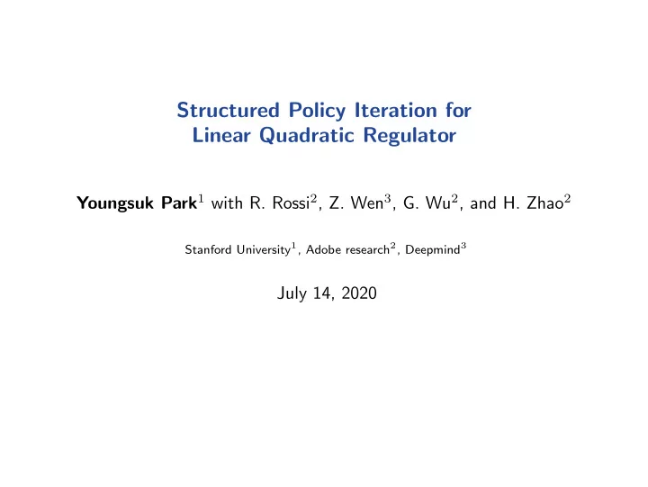
Structured Policy Iteration for Linear Quadratic Regulator Youngsuk Park 1 with R. Rossi 2 , Z. Wen 3 , G. Wu 2 , and H. Zhao 2 Stanford University 1 , Adobe research 2 , Deepmind 3 July 14, 2020

Introduction ◮ reinforcement learning (RL) is about learning from interaction with delayed feedback – decide action to take, which affects the next state of environment – need sequential decision making ◮ most of discrete RL algorithms scales poorly for tasks in continuous space – discretize state or/and action space – curse of dimensionality – sample inefficiency 2

Linear Quadratic Regulator ◮ Linear Quadratic Regulator (LQR) has rich applications for continuous space task – e.g., motion planning, trajectory optimization, portfolio ◮ Infinite horizon (undiscounted) LQR problem � ∞ � � x T t Qx t + u T E minimize t Ru t (1) π t =0 subject to x t +1 = Ax t + Bu t , u t = π ( x t ) , x 0 ∼ D , where A ∈ R n × n , B ∈ R n × m , Q � 0 , and R ≻ 0 . – quadratic cost Q, R and linear dynamics A, B – Q, R set relative weights of state deviation and input usage Preliminary 3

Linear Quadratic Regulator (Continued) ◮ LQR problem � ∞ � � x T t Qx t + u T minimize E t Ru t π t =0 subject to x t +1 = Ax t + Bu t , u t = π ( x t ) , x 0 ∼ D , where A ∈ R n × n , B ∈ R n × m , Q � 0 , and R ≻ 0 . ◮ well-known facts – linear optimal policy (or control gain) π ⋆ ( x ) = Kx, – quadratic optimal value function (cost-to-go) V ⋆ ( x ) = x T Px s.t. P = A T PA + Q − A T PB ( B T PB + R ) − 1 B T PA, K = − ( B T PB + R ) − 1 B T PA. – P can be derived efficiently, e.g., Riccati recursion, SDP, etc ◮ many variants and extensions – e.g., time-varying, averaged or discounted, jumping LQR etc. Preliminary 4

Structured Linear Policy ◮ can we find the structured linear policy for LQR? ◮ structure can mean (block) sparse, low-rank, etc – more interpretable, memory and computationally efficient, well-suited for distributed setting – Often, structure policy is related to physical decision system ◮ e.g., data cooling system need to install/arrange cooling infrastructure ◮ To tackle this, we develop – formulation, algorithm, theory and practice Preliminary 5

Formulation ◮ regularized LQR problem f ( K ) � �� � � ∞ � � x T t Qx t + u T minimize E t Ru t + λr ( K ) (2) K t =0 subject to x t +1 = Ax t + Bu t , u t = Kx t , x 0 ∼ D , – explicitly restrict policy to linear class, i.e., u t = Kx t – value function is still quadratic, i.e., V ( x ) = x T Px for some P – convex regularizer with (scalar) parameter λ ≥ 0 ◮ regularizer r ( K ) induces the policy structure – lasso � K � 1 = � i,j | K i,j | for sparse structure – group lasso � K � G , 2 = � g ∈G � K g � 2 for block-diagonal structure – nuclear-norm � K � ∗ = � i σ i ( K ) for low-rank structure F for some K ref ∈ R n × m , – proximity � K − K ref � 2 Preliminary 6

Structured Policy Iteration (S-PI) ◮ When model is known, S-PI repeats – (1) Policy (and covariance) evaluation ◮ solve Lyapunov equations to return ( P i , Σ i ) ( A + BK i ) T P i ( A + BK i ) − P i + Q + ( K i ) T RK i = 0 , ( A + BK i )Σ i ( A + BK i ) T − Σ i + Σ 0 = 0 . – (2) Policy improvement R + B T P i B K i + B T P i A ◮ compute gradient ∇ K f ( K i ) = 2 �� � � Σ i ◮ apply proximal gradient step under linesearch ◮ note that – Lyapunov equation requires O ( n 3 ) to solve – (almost) no hyperparameter to tune under linesearch (LS), – LS make stability ρ ( A + BK i ) < 1 satisfied Part 1: Model-based approach for regularized LQR 7

Convergence ’20) Assume K 0 s.t. K i from ρ ( A + BK 0 ) < 1 . Theorem (Park et al. S-PI Algorithm converges to the stationary point K ⋆ . Moreover, it converges linearly, i.e., after N iterations, � N � 2 � 1 − 1 � K N − K ⋆ � � � K 0 − K ⋆ � � 2 F ≤ F . � � � κ Here, κ = 1 / ( η min σ min (Σ 0 ) σ min ( R ))) > 1 where � σ min (Σ 0 ) , σ min ( Q ) , 1 η min = h η λ , 1 1 � R � , 1 1 1 � � A � , � B � , ∆ , , (3) F ( K 0 ) for some non-decreasing function h η on each argument. – Riccati recursion can give stabilizing initial policy K 0 – (global bound on) fixed stepsize η min depends on model parameters – note η min ∝ 1 /λ – in practice using LS, stepsize does have to be tuned or calculated Part 1: Model-based approach for regularized LQR 8

Model-free Structured Policy Iteration ◮ when model is unknown, S-PI repeats – (1) Perturbed policy evaluation N traj ◮ get perturbation and (perturbed) cost-to-go { ˆ f j , U j } j =1 for each j = 1 , . . . , N traj sample U j ∼ Uniform( S r ) to get a perturbed ˆ K i = K i + U j K i over the horizon H to estimate the cost-to-go roll out ˆ H f j = ˆ � g ( x t , ˆ K i x t ) t =0 – (2) Policy improvement ◮ compute the (noisy) gradient N traj 1 n � � r 2 ˆ f j U j ∇ K f ( K i ) = N traj j =1 ◮ apply proximal gradient step ◮ note that – smoothing procedure adapted to estimate noisy gradient – ( N traj , H, r ) are additional hyperparameters to tune – LS is not applicable Part 2: Model-free approach for regularized LQR 9

Convergence Theorem (Park et al. ’20) Suppose F ( K 0 ) is finite, Σ 0 ≻ 0 , and that x 0 ∼ D has norm bounded by D almost surly. Suppose the parameters in Algorithm ?? are chosen from D 2 � n, 1 1 � ( N traj , H, 1 /r ) = h ǫ , σ min (Σ 0 ) σ min ( R ) , . σ min (Σ 0 ) for some polynomials h . Then, with the same stepsize in Eq. (3), there exist � � K 0 − K ⋆ � F � � K N − K ⋆ � � � ≤ ǫ with iteration N at most 4 κ log such that ǫ at least 1 − o ( ǫ n − 1 ) probability. Moreover, it converges linearly, � i � � 1 − 1 � 2 ≤ � 2 , � K i − K ⋆ � � K 0 − K ⋆ � � 2 κ for the iteration i = 1 , . . . , N , where κ = ησ min (Σ 0 ) σ min ( R ) > 1 . – Assume K 0 is stabilizing policy but cannot use Riccati here – here ( N traj , H, r ) are hyperparameters to tune Part 2: Model-free approach for regularized LQR 10

Experiment (Setting) ◮ Consider unstable Laplacian system A ∈ R n × n where  1 . 1 , i = j   A ij = 0 . 1 , i = j + 1 or j = i + 1   0 , otherwise B = Q = I n ∈ R n × n and R = 1000 × I n ∈ R n × n . – unstable open loop system, i.e., ρ ( A ) ≥ 1 – extremely sensitive to parameters (even under known model setting) – less in favor of the generic model-free RL approaches to deploy ◮ Model and S-PI algorithm parameter under known model – system size n ∈ [3 , 500] – lasso penalty with λ ∈ [10 − 2 , 10 6 ] – LS with initial stepsize η = 1 λ with backtracking factor β = 1 2 � 1 � – For fixed stepsize, select η = O λ Experiment 11

Experiment (Continued) ◮ Convergence behavior under LS and scalability Convergence over differnt λ 100 10 −5 λ =588 λ =597 10 −7 λ =606 80 λ =615 10 −9 λ =624 time(sec) 60 f ( K i )/ f ( K ⋆ ) 10 −11 10 −13 40 10 −15 20 10 −17 10 −19 0 0 100 200 300 400 0 1 2 3 dimension n iteration i – S-PI with LS converges very fast over various n and λ – scales well for large system, even with computational bottleneck on solving Lyapunov equation – For n = 500 , takes less than 2 mins (MacBook Air) Experiment 12

Experiment (Continued) ◮ Dependency of stepsize η on λ . Largest fixed stetpsize with stable system 10 −5 stepsize η fixed 10 −6 10 3 10 4 10 5 λ – vary λ under same system – largest (fixed) stepsize for stable (closed) system, i.e., A + BK i < 1 is non-increasing, i.e., η fixed ∝ 1 λ Experiment 13

Experiment (Continued) ◮ Trade off between LQR performance and structure K The effect of different λ 1.0040 F ( K ⋆ )/ F ( K lqr ) 1.0035 1.0030 1.0025 590 610 630 card ( K ⋆ )/ card ( K lqr ) 1.00 0.75 0.50 0.25 590 610 630 λ – LQR solution K lqr , and S-PI solution K ⋆ – λ increases, LQR cost f ( K ⋆ ) increases whereas cardinality decreases (sparsitiy is improved). – In this range, S-PI barely changes LQR cost but improved the sparsity more than 50% . Experiment 14

Experiment (Continued) ◮ sparsity pattern of policy matrix λ = 600, card(K)=132 λ = 620, card(K)=62 0 5 10 15 0 5 10 15 0 0 5 5 10 10 15 15 – sparsity pattern (location of non-zero elements) of the policy matrix with λ = 600 and λ = 620 . Experiment 15

Challenge on model-free approach ◮ model-free approach is challenging and unstable – especially unstable open loop system ρ ( A ) < 1 – suffer similar difficulty to the model-free policy gradient method [Fazel et al., 2018] for LQR – finding stabilizing initial policy K 0 is non-trivial unless ρ ( A ) < 1 – suffer high variance, especially sensitive to smoothing parameter r ◮ open problems and algorithmic efforts needed in practice – variance reduction – rule of thumb to tune hyperparamters ◮ still, promising as a different class of model-free approach – no discretization – no need to compute Q ( s, a ) pair (like in REINFORCE) – seems to work for averaged cost of LQR (easier class of LQR) – more in longer version of paper Experiment 16