Stochastic Volatility Modeling Jean-Pierre Fouque University of - PowerPoint PPT Presentation

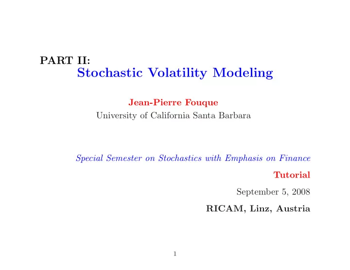
PART II: Stochastic Volatility Modeling Jean-Pierre Fouque University of California Santa Barbara Special Semester on Stochastics with Emphasis on Finance Tutorial September 5, 2008 RICAM, Linz, Austria 1

References: Derivatives in Financial Markets with Stochastic Volatility Cambridge University Press, 2000 Stochastic Volatility Asymptotics SIAM Journal on Multiscale Modeling and Simulation, 2(1), 2003 Collaborators: G. Papanicolaou (Stanford), R. Sircar (Princeton), K. Sølna (UCI) http://www.pstat.ucsb.edu/faculty/fouque 2

What is Volatility? Several notions of volatility Model dependent or not, Data dependent or not • Realized Volatility (historical data) • Model Volatility: – Local Volatility – Stochastic Volatility • Implied Volatility (option data) 3

Realized Volatility t 0 < t 1 < · · · < t N = t (present time) � � 2 � t N � log S t i − log S t i − 1 1 1 σ 2 s ds ∼ t − t 0 N t i − t i − 1 t 0 i =1 depends on the choice of t 0 and on the number of increments N (assuming t i − t i − 1 constant). More details: Zhang, L., Mykland, P.A., and Ait-Sahalia, Y. (2005). A tale of two time scales: Determining integrated volatility with noisy high-frequency data , J. Amer. Statist. Assoc. 100, 1394-1411. http://galton.uchicago.edu/˜mykland/publ.html 4

Volatility Models dS t = S t ( µdt + σ t dW t ) • Local Volatility: σ t = σ ( t, S t ) where σ ( t, x ) is a deterministic function. • Stochastic Volatility: σ t = f ( Y t ) where Y t contains an additional source of randomness. 5

Implied Volatility I ( t, T, K ) = σ implied ( t, T, K ) where σ implied ( t, T, K ) is uniquely defined by inverting Black-Scholes formula: C observed ( t, T, K ) = C BS ( t, S t ; T, K ; σ implied ( t, T, K )) given the call-option data. t is present time, T is the option maturity date, and K is the strike price. 6

0.4 0.35 9 Feb, 2000 0.3 Skew 0.25 Implied Volatility 0.2 0.15 Excess kurtosis Historical Volatility 0.1 0.05 0 0.8 0.85 0.9 0.95 1 1.05 1.1 Moneyness K/x Figure 1: S&P 500 Implied Volatility Curve as a function of moneyness from S&P 500 index options on February 9, 2000. The current index value is x = 1411 . 71 and the options have over two months to maturity. This is typically described as a downward sloping skew . 7

“Parametrization” of the Implied Volatility Surface I ( t ; T, K ) REQUIRED QUALITIES • Universal Parsimonous Parameters : Model Independence • Stability in Time : Predictive Power • Easy Calibration : Practical Implementation • Compatibility with Price Dynamics : Applicability to Pricing other Derivatives and Hedging 8

At least three approaches: • Local Volatility Models : σ t = σ ( t, S t ) +’s: market is complete (no additional randomness), Dupire formula ∂C ∂T + rK ∂C σ 2 ( T, K ) ∂K = 2 K 2 ∂ 2 C ∂K 2 -’s: stability of calibration • Implied Volatility Surface Models : dI t ( T, K ) = · · · +’s: predictive power -’s: no-arbitrage conditions not easy. Which underlying? • Stochastic Volatility Models : σ t = f ( Y t ) 9

Stochastic Volatility Framework WHY? • Distributions of returns are not log-normal • Smile (Skew) effect observed in implied volatilities HOW? dS t = µS t dt + σ t S t dW t with, for instance: σ t = f ( Y t ) √ 2 α dW (1) dY t = α ( m − Y t ) dt + ν t d � W, W (1) � t = ρdt 10

The Popular Heston Model µS t dt + σ t S t dW (1) dS t = t � σ t = Y t � 2 αY t dW (2) dY t = α ( m − Y t ) dt + ν t d � W (1) , W (2) � t = ρdt t Y t is a CIR (Cox-Ingersoll-Ross) process. The condition m ≥ ν 2 ensures that the process Y t stays strictly positive at all time. 11

Mean-Reverting Stochastic Volatility Models dX t = X t ( µdt + σ t dW t ) σ t = f ( Y t ) For instance: 0 < σ 1 ≤ f ( y ) ≤ σ 2 for every y dY t = α ( m − Y t ) dt + β ( · · · ) d ˆ Z t Brownian motion ˆ Z correlated to W : � ˆ 1 − ρ 2 Z t , Z t = ρW t + | ρ | < 1 so that d � W, ˆ Z � t = ρdt 12

Pricing under Stochastic Volatility P ⋆ ( γ ) Risk-neutral probability chosen by the market: I rX t dt + f ( Y t ) X t dW ⋆ dX t = t � � �� � ρ ( µ − r ) dt + βd ˆ Z ⋆ 1 − ρ 2 dY t = α ( m − Y t ) − β f ( Y t ) + γ t � ˆ 1 − ρ 2 Z ⋆ Z ⋆ ρW ⋆ = t + t t Market price of volatility risk: γ = γ ( y ) E ⋆ ( γ ) { e − r ( T − t ) h ( X T ) |F t } P t = I Markovian case: E ⋆ ( γ ) { e − r ( T − t ) h ( X T ) | X t = x, Y t = y } P ( t, x, y ) = I but y (or f ( y ) ) is not directly observable! 13

Stochastic Volatility Pricing PDE 2 f ( y ) 2 x 2 ∂ 2 P ∂x 2 + ρβxf ( y ) ∂ 2 P 2 β 2 ∂ 2 P ∂P ∂t + 1 ∂x∂y + 1 ∂y 2 � � x∂P + α ( m − y ) ∂P ∂y − β Λ ∂P + r ∂x − P = 0 ∂y where � Λ = ρ ( µ − r ) 1 − ρ 2 + γ f ( y ) Terminal condition: P ( T, x, y ) = h ( x ) No perfect hedge! 14

Summary of the stochastic volatility approach Positive aspects: • More realistic returns distributions (fat tails and asymmetry ) • Smile effect with skew contolled by ρ Difficulties: • Volatility not directly observed, parameter estimation difficult • No canonical model. Relevance of explicit formulas? • Incomplete markets, no perfect hedge • Volatility risk premium to be estimated from option prices • Numerical difficulties due to higher dimension 15

Fast Mean-Reverting Stochastic Volatility Asymptotic Analysis 16

P ⋆ ( γ ) in terms of ε = 1 /α Model in the risk-neutral world I √ √ ε so that ν 2 = β 2 / 2 α Set β = ν 2 dX ε rX ε t dt + f ( Y ε t ) X ε t dW ⋆ = t t � � √ √ 1 t ) − ν 2 dt + ν 2 √ ε d ˆ dY ε ε ( m − Y ε √ ε Λ( Y ε Z ⋆ = t ) t t Market price of risks: � Λ( y ) = ρ ( µ − r ) 1 − ρ 2 + γ ( y ) f ( y ) Skew: � ˆ Z ⋆ t = ρW ⋆ 1 − ρ 2 Z ⋆ t + , | ρ | < 1 t 17

Prices and Pricing PDE’s E ⋆ ( γ ) � � P ε ( t, x, y ) = I e − r ( T − t ) h ( X ε T ) | X ε t = x, Y ε t = y √ ∂P ε 2 f ( y ) 2 x 2 ∂ 2 P ε √ ε xf ( y ) ∂ 2 P ε ∂x∂y + ν 2 ∂ 2 P ε ∂t + 1 ∂x 2 + ρν 2 ∂y 2 ε √ � � x∂P ε ε ( m − y ) ∂P ε √ ε Λ( y ) ∂P ε + 1 ∂y − ν 2 ∂x − P ε + r = 0 ∂y to be solved for t < T with the terminal condition P ε ( T, x, y ) = h ( x ) 18

Operator Notation � 1 � ε L 0 + 1 P ε = 0 √ ε L 1 + L 2 with ν 2 ∂ 2 ∂y 2 + ( m − y ) ∂ L 0 = = L OU ∂y √ √ 2 ρνxf ( y ) ∂ 2 2 ν Λ( y ) ∂ L 1 = ∂x∂y − ∂y � � 2 f ( y ) 2 x 2 ∂ 2 ∂t + 1 ∂ x ∂ L 2 = ∂x 2 + r ∂x − · = L BS ( f ( y )) 19

Formal Expansion Expand: P ε = P 0 + √ εP 1 + εP 2 + ε √ εP 3 + · · · Compute: � 1 � � � P 0 + √ εP 1 + εP 2 + ε √ εP 3 + · · · ε L 0 + 1 √ ε L 1 + L 2 = 0 Group the terms by powers of ε : 1 1 √ ε ( L 0 P 1 + L 1 P 0 ) ε L 0 P 0 + + ( L 0 P 2 + L 1 P 1 + L 2 P 0 ) √ ε ( L 0 P 3 + L 1 P 2 + L 2 P 1 ) + + · · · = 0 20

Diverging terms • Order 1 /ε : L 0 P 0 = 0 L 0 = L OU , acting on y = ⇒ P 0 = P 0 ( t, x ) with P 0 ( T, x ) = h ( x ) • Order 1 / √ ε : L 0 P 1 + L 1 P 0 = 0 L 1 takes derivatives w.r.t. y = ⇒ L 1 P 0 = 0 = ⇒ L 0 P 1 = 0 As for P 0 : P 1 = P 1 ( t, x ) P 1 ( T, x ) = 0 with • Important observation: P 0 + √ εP 1 does not depend on y 21

Zero Order Term L 0 P 2 + ( L 1 P 1 = 0) + L 2 P 0 = 0 Poisson equation in P 2 with respect to L 0 and the variable y . Solution: P 2 = ( −L 0 ) − 1 ( L 2 P 0 ) Only if L 2 P 0 is centered with respect to the invariant distribution of Y . 22

Poisson Equations L 0 χ + g = 0 Expectations w.r.t. the invariant distribution of the OU process: � � χ ( y )( L ⋆ � g � = −�L 0 χ � = − ( L 0 χ ( y ))Φ( y ) dy = 0 Φ( y )) dy = 0 t → + ∞ I lim E { g ( Y t ) | Y 0 = y } = � g � = 0 (exponentially fast) � + ∞ χ ( y ) = I E { g ( Y t ) | Y 0 = y } dt 0 checked by applying L 0 23

Leading Order Term Centering: �L 2 P 0 � = �L 2 � P 0 = 0 � ∂ � �� 2 f ( y ) 2 x 2 ∂ 2 ∂t + 1 x ∂ �L 2 � = ∂x 2 + r ∂x − · � � 2 � f 2 � x 2 ∂ 2 ∂t + 1 ∂ x ∂ = ∂x 2 + r ∂x − · � f 2 � σ 2 = Effective volatility: ¯ The zero order term P 0 ( t, x ) is the solution of the Black-Scholes equation L BS (¯ σ ) P 0 = 0 with the terminal condition P 0 ( T, x ) = h ( x ) 24

Back to P 2 ( t, x, y ) The centering condition �L 2 P 0 � = 0 being satisfied: � σ 2 � x 2 ∂ 2 P 0 L 2 P 0 = L 2 P 0 − �L 2 P 0 � = 1 f ( y ) 2 − ¯ ∂x 2 2 2 L 0 φ ( y ) x 2 ∂ 2 P 0 = 1 ∂x 2 for φ a solution of the Poisson equation: L 0 φ = f ( y ) 2 − � f 2 � Then 2 ( φ ( y ) + c ( t, x )) x 2 ∂ 2 P 0 ( L 2 P 0 ) = − 1 P 2 ( t, x, y ) = −L − 1 0 ∂x 2 25

Terms of order √ ε Poisson equation in P 3 : L 0 P 3 + L 1 P 2 + L 2 P 1 = 0 Centering condition: �L 1 P 2 + L 2 P 1 � = 0 Equation for P 1 : � � �� ( φ ( y ) + c ( t, x )) x 2 ∂ 2 P 0 �L 2 P 1 � = −�L 1 P 2 � = 1 L 1 ∂x 2 2 P 1 independent of y and L 1 takes derivatives w.r.t. y � � x 2 ∂ 2 P 0 σ ) P 1 = 1 = ⇒ L BS (¯ 2 �L 1 φ ( y ) � ∂x 2 with P 1 ( T, x ) = 0 26