Stochastic Simulation Testing random number generaters Bo Friis - PowerPoint PPT Presentation

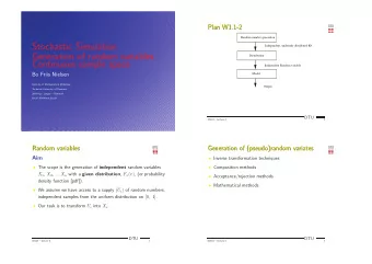
Stochastic Simulation Testing random number generaters Bo Friis Nielsen Applied Mathematics and Computer Science Technical University of Denmark 2800 Kgs. Lyngby – Denmark Email: bfn@imm.dtu.dk

Testing random number generaters Testing random number generaters • Theoretical tests/properties • Tests for uniformity • Tests for independence DTU 02443 – lecture 2 2

Characteristics of random number generators Characteristics of random number generators Definition: A sequence of pseudo-random numbers U i is a deterministic sequence of numbers in ]0 , 1[ having the same relevant statistical properties as a sequence of random numbers. The question is what are relevant statistical properties. • Distribution type • Randomness (independence, whiteness) DTU 02443 – lecture 2 3

Theoretical tests/properties Theoretical tests/properties • Test of global behaviour (entire cycles) • Mathematical theorems • Typically investigates multidimensional uniformity DTU 02443 – lecture 2 4

Testing random number generators Testing random number generators • Test for distribution type ⋄ Visual tests/plots ⋄ χ 2 test ⋄ Kolmogorov Smirnov test • Test for independence ⋄ Visual tests/plots ⋄ Run test up/down ⋄ Run test length of runs ⋄ Test of correlation coefficients DTU 02443 – lecture 2 5

Significance test Significance test • We assume (known) model - The hypothesis • We identify a certain characterising random variable - The test statistic • We reject the hypothesis if the test statistic is an abnormal observation under the hypothesis DTU 02443 – lecture 2 6

Key terms Key terms • Hypothesis/Alternative • Test statistic • Significance level • Accept/Critical area • Power • p -value DTU 02443 – lecture 2 7

Multinomial distribution Multinomial distribution • n items • k classes • each item falls in class j with probabibility p j • X j is the (random) number of items in class j • We write X = ( X 1 , . . . , X 2 ) ∼ Mul ( n, p 1 , . . . , p k ) Thus X j ∼ Bin ( n, p j ) E ( X j ) = np j , Var ( X j ) = np j (1 − p j ) � � � � X j − np j X j − np j √ √ And E = 0 Var = 1 np j (1 − p j ) np j (1 − p j ) n →∞ X j − np j √ Thus ∼ N (0 , 1) np j (1 − p j ) DTU 02443 – lecture 2 8

Test statistic for k − 2 Test statistic for k − 2 n →∞ X j − np j √ Recall ∼ N (0 , 1) np j (1 − p j ) � 2 � = ( X j − np j ) 2 asymp X j − np j √ χ 2 (1) thus ∼ np j (1 − p j ) np j (1 − p j ) Consider now the case k = 2 ( X 1 − np 1 ) 2 np 1 (1 − p 1 ) = ( X 1 − np 1 ) 2 ( p 1 +1 − p 1 ) = ( X 1 − np 1 ) 2 + ( X 1 − np 1 ) 2 np 1 (1 − p 1 ) np 1 n (1 − p 1 ) = ( X 1 − np 1 ) 2 + ( X 1 − n − n ( p 1 − 1)) 2 = ( X 1 − np 1 ) 2 + ( − X 2 + np 2 ) 2 n (1 − p 1 ) np 1 np 1 np 2 = ( X 1 − np 1 ) 2 + ( X 2 − np 2 ) 2 np 1 np 2 • the χ 2 statistic • the proof can be completed by induction DTU 02443 – lecture 2 9

Test for distribution type χ 2 test Test for distribution type χ 2 test The general form of the test statistic is n classes ( n observed ,i − n expected ,i ) 2 � T = n expected ,i i =1 • The test statistic is to be evaluated with a χ 2 distribution with f degrees of freedom. d f is generally n classes − 1 − m where m d is the number of estimated parameters. • It is recommend to choose all groups such that n expected ,i ≥ 5 DTU 02443 – lecture 2 10

Test for distribution type Kolmogorov Smirnov Test for distribution type Kolmogorov Smirnov test test • Compare empirical distribution function F n ( x ) with hypothesized distribution F ( x ) . • For known parameters the test statistic does not depend on F ( x ) • Better power than the χ 2 test • No grouping considerations needed • Works only for completely specified distributions in the original version DTU 02443 – lecture 2 11

Empirical distribution Empirical distribution 20 N (0 , 1) variates (sorted): -2.20, -1.68, -1.43, -0.77, -0.76, -0.12, 0.30, 0.39, 0.41, 0.44, 0.44, 0.71, 0.85, 0.87, 1.15, 1.37, 1.41, 1.81, 2.65, 3.69 X i iid random variables with F ( x ) = P ( X ≤ x ) Each leads to a (simple) random function F e,i ( x ) = 1 { X i ≤ x } � n � n leading to F e ( x ) = 1 i =1 F e,i ( x ) = 1 i =1 1 { X i ≤ x } n n � 1 � n � n = 1 � � � E ( F e ( x )) = E i =1 E = F ( x ) i =1 1 { X i ≤ x } 1 { X i ≤ x } n n n 2 nF ( x )(1 − F ( x )) = F ( x ) G ( x ) 1 Var ( F e ( x )) = n � � n →∞ F ( x ) , F ( x ) G ( x ) F e ( x ) ∼ N n In the limit ( n → ∞ ) we have a random continuous function of x - a stochastic process, more particularly a Brownian bridge DTU 02443 – lecture 2 12

Empirical distribution Empirical distribution 20 N (0 , 1) variates (sorted): -2.20, -1.68, -1.43, -0.77, -0.76, -0.12, 0.30, 0.39, 0.41, 0.44, 0.44, 0.71, 0.85, 0.87, 1.15, 1.37, 1.41, 1.81, 2.65, 3.69 D n = sup x {| F n ( x ) − F ( x ) |} the test statistic follows Kolmogorovs distribution

Test statistic and significance levels Test statistic and significance levels Level of significance (1 − α ) Case Adjusted test statistic 0.850 0.900 0.950 0.975 0.990 � √ n + 0 . 12 + 0 . 11 � All parameters known D n 1.138 1.224 1.358 1.480 1.628 √ n � √ n − 0 . 01 + 0 . 85 � N ( ¯ X ( n ) , S 2 ( n )) D n 0.775 0.819 0.895 0.955 1.035 √ n � √ n + 0 . 26 + 0 . 5 � � exp( ¯ D n − 0 . 2 � X ( n )) 0.926 0.990 1.094 1.190 1.308 √ n n DTU

Test for correlation - Visual tests Test for correlation - Visual tests • Plot of U i +1 versus U i Random numbers U_i against U_{i+1}, X_{i+1} = (5 X_i + 1)(mod 16) Random numbers U_i against U_{i+1}, X_{i+1} = (129 X_i + 26461)(mod 65536) 1 1 ’ranplot.lst’ ’ranplot2.lst’ 0.9 0.9 0.8 0.8 0.7 0.7 0.6 0.6 0.5 0.5 0.4 0.4 0.3 0.3 0.2 0.2 0.1 0.1 0 0 0 0.1 0.2 0.3 0.4 0.5 0.6 0.7 0.8 0.9 1 0 0.1 0.2 0.3 0.4 0.5 0.6 0.7 0.8 0.9 1 DTU 02443 – lecture 2 15

Indepedence test: Test for multidimensional Indepedence test: Test for multidimensional uniformity uniformity • In the two dimensional version test for uniformity of ( U 2 i − 1 , U 2 i ) • Typically χ 2 test • The number of groups increases drastically with dimension DTU 02443 – lecture 2 16

Run test I Run test I Above/below • The run test given in Conradsen, can be used by e.g. comparing with the median. • The number of runs (above/below the median) is (asymptotically) distributed as � + 1 , 2 n 1 n 2 (2 n 1 n 2 − n 1 − n 2 ) � 2 n 1 n 2 N ( n 1 + n 2 ) 2 ( n 1 + n 2 − 1) n 1 + n 2 where n 1 is the number of samples above and n 2 is the number below. • The test statistic is the total number of runs T = R a + R b with R a (runs above) and R b (runs below) DTU 02443 – lecture 2 17

Run tests II Run tests II Up/Down from Knuth A test specifically designed for testing random number generators is the following UP/DOWN run test, see e.g. Donald E. Knuth, The Art of Computer Programming Volume 2, 1998, pp. 66-. The sequence: 0 . 54 , 0 . 67 , | 0 . 13 , 0 . 89 , | 0 . 33 , 0 . 45 , 0 . 90 , | 0 . 01 , 0 . 45 , 0 . 76 , 0 . 82 , | 0 . 24 , | 0 . 17 has runs of length 2,2,3,4,1, ... i.e. runs of consecutively increa- sing numbers. DTU 02443 – lecture 2 18

Run test II Run test II Generate n random numbers.The observed number of runs of length 1 , . . . , 5 and ≥ 6 are recorded in the vector R . The test statistic is calculated by: 1 n − 6( R − n B ) T A ( R − n B ) Z =     1 4529 . 4 9044 . 9 13568 18091 22615 27892 6     5 9044 . 9 18097 27139 36187 45234 55789     24         11 13568 27139 40721 54281 67852 83685     120 A = B =         19 18091 36187 54281 72414 90470 111580     720     29     22615 45234 67852 90470 113262 139476     5040     1 27892 55789 83685 111580 139476 172860 840 The test statistic is compared with a χ 2 (6) distribution. One should have n > 4000

Run test III Run test III The-Up-and-Down Test This test is described in Rubinstein 81 “Simulation and the Monte Carlo Method” and Iversen 07 (in Danish). The sequence: 0 . 54 , 0 . 67 , 0 . 13 , 0 . 89 , 0 . 33 , 0 . 45 , 0 . 90 , 0 . 01 , 0 . 45 , 0 . 76 , 0 . 82 , 0 . 24 , 0 . 17 is converted to <, >, <, >, <, <, >, <, <, <, >, > giving in total 8 runs of length 1 , 1 , 1 , 1 , 2 , 1 , 3 , 2 DTU 02443 – lecture 2 20

Run test III Run test III The expected number of runs of length k is n +1 12 , 11 n − 4 for runs of 12 length 1 and 2 respectively, and 2[( k 2 + 3 k + 1) n − ( k 3 + 3 k 2 − k − 4)] ( k + 3)! for runs of length k < N − 1 . Define X to be the total number of runs, then Z = X − 2 n − 1 3 � 16 n − 29 90 is asymptotically N(0,1). DTU 02443 – lecture 2 21

Correlation coefficients Correlation coefficients • the estimated correlation n − h 1 � 7 � � c h = U i U i + h ∼ N 0 . 25 , n − h 144 n i =1 DTU 02443 – lecture 2 22