Stochastic Processes MATH5835, P. Del Moral UNSW, School of - PowerPoint PPT Presentation
Stochastic Processes MATH5835, P. Del Moral UNSW, School of Mathematics & Statistics Lectures Notes No. 11 Consultations (RC 5112): Wednesday 3.30 pm 4.30 pm & Thursday 3.30 pm 4.30 pm 1/33 Reminder + Information References in
Stochastic Processes MATH5835, P. Del Moral UNSW, School of Mathematics & Statistics Lectures Notes No. 11 Consultations (RC 5112): Wednesday 3.30 pm � 4.30 pm & Thursday 3.30 pm � 4.30 pm 1/33
Reminder + Information References in the slides ◮ Material for research projects � Moodle ( Stochastic Processes and Applications ∋ variety of applications) 2/33
– Richard P. Feynman (1918-1988) ⊕ video 3/33
Three objectives Understanding & Solving ◮ Classical stochastic algorithms ◮ Some advanced Monte Carlo schemes ◮ Intro to computational physics/biology 4/33
Plan of the lecture ◮ Stochastic algorithms ◮ Robbins Monro model ◮ Simulated annealing 5/33
Plan of the lecture ◮ Stochastic algorithms ◮ Robbins Monro model ◮ Simulated annealing ◮ Some advanced Monte Carlo models ◮ Interacting simulated annealing ◮ Rare event sampling ◮ Black box and inverse problems 5/33
Plan of the lecture ◮ Stochastic algorithms ◮ Robbins Monro model ◮ Simulated annealing ◮ Some advanced Monte Carlo models ◮ Interacting simulated annealing ◮ Rare event sampling ◮ Black box and inverse problems ◮ Computational physics/biology ◮ Molecular dynamics ◮ Sch¨ odinger ground states ◮ Genetic type algorithms 5/33
Robbins Monro model Objectives Given U : R d �→ R d ∋ a U a = { x ∈ R d : U ( x ) = a } find 6/33
Robbins Monro model Objectives Given U : R d �→ R d ∋ a U a = { x ∈ R d : U ( x ) = a } find Examples ◮ Concentration of products (therapeutic,...): U ( x ) = E ( U ( x , Y )) U ( x , Y ) := U (”drug” dose x , ”data” patients Y ) = dosage effects 6/33
Robbins Monro model Objectives Given U : R d �→ R d ∋ a U a = { x ∈ R d : U ( x ) = a } find Examples ◮ Concentration of products (therapeutic,...): U ( x ) = E ( U ( x , Y )) U ( x , Y ) := U (”drug” dose x , ”data” patients Y ) = dosage effects ◮ Median and quantiles estimation U ( x ) = P ( Y ≤ x ) find x a s.t. P ( Y ≤ x a ) = a � 6/33
Robbins Monro model Objectives Given U : R d �→ R d ∋ a U a = { x ∈ R d : U ( x ) = a } find Examples ◮ Concentration of products (therapeutic,...): U ( x ) = E ( U ( x , Y )) U ( x , Y ) := U (”drug” dose x , ”data” patients Y ) = dosage effects ◮ Median and quantiles estimation U ( x ) = P ( Y ≤ x ) find x a s.t. P ( Y ≤ x a ) = a � ◮ Optimization problems ( V smooth & convex) U ( x ) = ∇ V ( x ) find x 0 s.t. ∇ V ( x 0 ) = 0 � 6/33
When U is known Hypothesis U a = { x a } & � ( x − x a ) , U ( x ) − U ( x a ) � > 0 7/33
When U is known Hypothesis U a = { x a } & � ( x − x a ) , U ( x ) − U ( x a ) � > 0 � d = 1 Same sign! U ( x ) ≥ U ( x a ) ⇒ x ≥ x a U ( x ) ≤ U ( x a ) ⇒ x ≤ x a 7/33
When U is known Hypothesis U a = { x a } & � ( x − x a ) , U ( x ) − U ( x a ) � > 0 � d = 1 Same sign! U ( x ) ≥ U ( x a ) ⇒ x ≥ x a U ( x ) ≤ U ( x a ) ⇒ x ≤ x a Algorithm? 7/33
When U is known Hypothesis U a = { x a } & � ( x − x a ) , U ( x ) − U ( x a ) � > 0 � d = 1 Same sign! U ( x ) ≥ U ( x a ) ⇒ x ≥ x a U ( x ) ≤ U ( x a ) ⇒ x ≤ x a Algorithm? x n +1 = x n + γ n ( U ( x a ) − U ( x n )) 7/33
When U is known Hypothesis U a = { x a } & � ( x − x a ) , U ( x ) − U ( x a ) � > 0 � d = 1 Same sign! U ( x ) ≥ U ( x a ) ⇒ x ≥ x a U ( x ) ≤ U ( x a ) ⇒ x ≤ x a Algorithm? x n +1 = x n + γ n ( U ( x a ) − U ( x n )) with some technical conditions � � γ 2 γ n = ∞ and n < ∞ n n 7/33
When U ( x ) = E ( U ( x , Y )) is un known Examples ◮ Quantiles U ( x ) = P ( Y ≤ x ) = E ( U ( x , Y )) U ( x , Y ) := 1 ] −∞ , x ] ( Y ) 8/33
When U ( x ) = E ( U ( x , Y )) is un known Examples ◮ Quantiles U ( x ) = P ( Y ≤ x ) = E ( U ( x , Y )) U ( x , Y ) := 1 ] −∞ , x ] ( Y ) ◮ Dosage effects Y = absorption curves of drugs w.r.t. time U ( x ) = E ( U ( x , Y )) 8/33
When U ( x ) = E ( U ( x , Y )) is un known Examples ◮ Quantiles U ( x ) = P ( Y ≤ x ) = E ( U ( x , Y )) U ( x , Y ) := 1 ] −∞ , x ] ( Y ) ◮ Dosage effects Y = absorption curves of drugs w.r.t. time U ( x ) = E ( U ( x , Y )) ◮ Noisy measurements x − → sensor/black box − → U ( x , Y ) := U ( x ) + Y 8/33
Un known � Sampling Ideal deterministic algorithm 9/33
Un known � Sampling Ideal deterministic algorithm x n +1 = x n + γ n ( U ( x a ) − U ( x n )) = x n + γ n ( a − U ( x n )) 9/33
Un known � Sampling Ideal deterministic algorithm x n +1 = x n + γ n ( U ( x a ) − U ( x n )) = x n + γ n ( a − U ( x n )) with some technical conditions � � γ 2 γ n = ∞ and n < ∞ n n 9/33
Un known � Sampling Ideal deterministic algorithm x n +1 = x n + γ n ( U ( x a ) − U ( x n )) = x n + γ n ( a − U ( x n )) with some technical conditions � � γ 2 γ n = ∞ and n < ∞ n n Robbins Monro algorithm X n +1 = X n + γ n ( a − U ( x n , Y n )) 9/33
Stochastic gradient Robbins Monro algorithm X n +1 = X n + γ n ( a − U ( x n , Y n )) 10/33
Stochastic gradient Robbins Monro algorithm X n +1 = X n + γ n ( a − U ( x n , Y n )) ⇓ a = 0 & U ( x , Y n ) = ∇V x ( x , Y n ) ( � U ( x ) = ∇ x E ( V x ( x , Y ))) 10/33
Stochastic gradient Robbins Monro algorithm X n +1 = X n + γ n ( a − U ( x n , Y n )) ⇓ a = 0 & U ( x , Y n ) = ∇V x ( x , Y n ) ( � U ( x ) = ∇ x E ( V x ( x , Y ))) Stochastic gradient X n +1 = X n − γ n ∇V x ( X n , Y n ) ���� learning rate 10/33
Example (linear regression) N data set z i ∈ R d � observation y i ∈ R d ′ Best x ∈ R d ? such that � y i ≃ h x ( z i ) + N (0 , 1) with h x ( z ) = x i z i 1 ≤ i ≤ d 11/33
Example (linear regression) N data set z i ∈ R d � observation y i ∈ R d ′ Best x ∈ R d ? such that � y i ≃ h x ( z i ) + N (0 , 1) with h x ( z ) = x i z i 1 ≤ i ≤ d Averaging criteria � � � I unif ∈{ 1 ,..., N } � h x ( z i ) − y i � 2 1 V ( x , ( y I , z I )) U ( x ) = E = = = = = = = = = = 2 N 1 ≤ i ≤ N with � h x ( z i ) − y i � z i � h x ( z i ) − y i � 2 ⇒ ∇ x V = V ( x , ( y i , z i )) = 1 1 . . . � h x ( z i ) − y i � 2 z i d 11/33
Example (linear regression) N data set z i ∈ R d � observation y i ∈ R d ′ Best x ∈ R d ? such that � y i ≃ h x ( z i ) + N (0 , 1) with h x ( z ) = x i z i 1 ≤ i ≤ d Averaging criteria � � � I unif ∈{ 1 ,..., N } � h x ( z i ) − y i � 2 1 V ( x , ( y I , z I )) U ( x ) = E = = = = = = = = = = 2 N 1 ≤ i ≤ N with � h x ( z i ) − y i � z i � h x ( z i ) − y i � 2 ⇒ ∇ x V = V ( x , ( y i , z i )) = 1 1 . . . � h x ( z i ) − y i � 2 z i d Stochastic gradient process X n − γ n ∇ x V ( X n , ( Y I n , Z I n ) X n +1 = 11/33
Simulated annealing Objectives V ⋆ = { x ∈ S : V ( x ) = inf given V : S �→ R find y V ( y ) } 12/33
Simulated annealing Objectives V ⋆ = { x ∈ S : V ( x ) = inf given V : S �→ R find y V ( y ) } � Probabilist viewpoint: ⇔ Sampling the Boltzmann-Gibbs distribution µ β ( dx ) := 1 e − β V ( x ) λ ( dx ) Z β for some reference measure λ . 12/33
Simulated annealing Objectives V ⋆ = { x ∈ S : V ( x ) = inf given V : S �→ R find y V ( y ) } � Probabilist viewpoint: ⇔ Sampling the Boltzmann-Gibbs distribution µ β ( dx ) := 1 e − β V ( x ) λ ( dx ) Z β for some reference measure λ . A couple of examples λ ( x i ) = 1 { x 1 , . . . , x k } λ ( { x i } ) S = := � d 1 ≤ i ≤ k dx i = Lebesgue measure on R k R k S = λ ( dx ) := 12/33
Optimization vs. Sampling Finite state spaces S = { x 1 , . . . , x k } ∋ x i e − β V ( x i ) λ ( x i ) e − β V ( x i ) µ β ( x i ) := � y ∈ S e − β V ( y ) λ ( y ) = � 1 ≤ j ≤ k e − β V ( x j ) 13/33
Optimization vs. Sampling Finite state spaces S = { x 1 , . . . , x k } ∋ x i e − β V ( x i ) λ ( x i ) e − β V ( x i ) µ β ( x i ) := � y ∈ S e − β V ( y ) λ ( y ) = � 1 ≤ j ≤ k e − β V ( x j ) Proposition 1 µ β ( x i ) − → β ↑∞ µ ∞ ( x i ) = Card ( V ⋆ ) 1 V ⋆ ( x i ) Proof: 13/33
Metropolis-Hastings transition Reversible proposition w.r.t. λ (local moves/neighbors) λ ( x ) P ( x , y ) = λ ( y ) P ( y , x ) 14/33
Metropolis-Hastings transition Reversible proposition w.r.t. λ (local moves/neighbors) λ ( x ) P ( x , y ) = λ ( y ) P ( y , x ) Acceptance/rejection transition � � 1 , µ β ( y ) P ( y , x ) M β ( x , y ) = P ( x , y ) min + . . . δ x ( dy ) µ β ( x ) P ( x , y ) P ( x , y ) e − β ( V ( y ) − V ( x )) + + . . . δ x ( dy ) = ⇓ 14/33
Metropolis-Hastings transition Reversible proposition w.r.t. λ (local moves/neighbors) λ ( x ) P ( x , y ) = λ ( y ) P ( y , x ) Acceptance/rejection transition � � 1 , µ β ( y ) P ( y , x ) M β ( x , y ) = P ( x , y ) min + . . . δ x ( dy ) µ β ( x ) P ( x , y ) P ( x , y ) e − β ( V ( y ) − V ( x )) + + . . . δ x ( dy ) = ⇓ Balance/Reversibility equation µ β ( y ) M β ( y , x ) = µ β ( x ) M β ( x , y ) 14/33
Recommend
More recommend
Explore More Topics
Stay informed with curated content and fresh updates.
