Simulated Annealing input : ( x 1 , t 1 ) , . . . , ( x N , t N ) R - - PowerPoint PPT Presentation

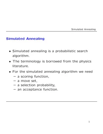
Simulated Annealing

input : (x1, t1), . . . , (xN, tN) ∈

Rd × {−1, +1}; Tstart, Tstop ∈ R

• utput: w

begin Randomly initialize w

T ← Tstart

repeat

• w ← N(w) //neighbors of w, e.g. by adding

Gaussion noise (N(0, σ)) if E(

w) < E(w) then w ← w

else if exp

• −E(b

w)−E(w) T

• > rand[0, 1) then

w ← w

decrease (T) until T < Tstop return w end

– p. 156

Continuous Hopfield Network

Let us consider our previously defined Hopfield network (identical architecture and learning rule), however with following activity rule

Si = tanh   1 T ·

• j

wijSj  

Start with a large (temperature) value of T and decrease it by some magnitude whenever a unit is updated (deterministic simulated annealing). This type of Hopfield network can approximate the probability distribution

P(x|W) = 1 Z(W) exp[−E(x)] = 1 Z(W) exp 1 2xTWx

• – p. 157

Continuous Hopfield Network

Z(W) =

• x′

exp(−E(x′))

(sum over all possible states) is the partition function and ensures P(x|W) is a probability distribution. Idea: construct a stochastic Hopfield network that implements the probability distribution P(x|W).

• Learn a model that is capable of generating patterns

from that unknown distribution.

• Quantify (classify) by means of probabilities seen and

unseen patterns.

• If needed, we can generate more patterns (generative

model).

– p. 158

Boltzmann Machines

Given patterns {x(n)}N

1 , we want to learn the weights such

that the generative model

P(x|W) = 1 Z(W) exp 1 2xTWx

• is well matched to those patterns. The states are updated

according to the stochastic rule:

• set xn = +1 with probability

1 1+exp (−2 P

j wijxj)

• else set xn = −1.

Posterior probability of the weights given the data (Bayes’ theorem)

P(W|{x(n)}N

1 ) =

N

n=1 P(x(n)|W)

• P(W)

P({x(n)}N

1 )

– p. 159

Boltzmann Machines

Apply maximum likelihood method on the first term in numerator:

ln N

• n=1

P(x(n)|W)

• =

N

• n=1

1 2x(n)T Wx(n) − ln Z(W)

• Taking derivative of the log likelihood gives: note that W is

symmetric (wij = wji) that is

∂ ∂wij 1 2x(n)T Wx(n) = x(n) i

x(n)

j

and ∂

∂wij ln Z(W) = 1 Z(w)

• x

∂ ∂wij exp 1 2x(n)T Wx(n)

• =

1 Z(W)

• x

exp 1 2x(n)T Wx(n)

• xixj

=

• x

xixj P(x|W) = xixjP(x|W)

– p. 160

Boltzmann Machines (cont.)

∂ ∂wij ln P({x(n)}N

1 |W)

=

N

• n=1
• x(n)

i

x(n)

j

− xixjP(x|W)

• =

N

• xixjData − xixjP(x|W)
• Empirical correlation between xi and xj

xixjData ≡ 1 N

N

• n=1
• x(n)

i

x(n)

j

• Correlation between xi and xj under the current model

xixjP(x|W) ≡

• x

xixjP(x|W)

– p. 161

Interpretation of Boltzmann Machines Learning

Illustrative description (MacKay’s book, pp. 523):

• Awake state: measure correlation between xi and xj in

the real world, and increase the weights in proportion to the measured correlations.

• Sleep state: dream about the world using the

generative model P(x|W) and measure the correlation between xi and xj in the model world. Use these correlations to determine a proportional decrease in the weights. If correlations in dream world and real world are matching, then the two terms balanced and weights do not change.

– p. 162

Boltzmann Machines with Hidden Units

To model higher order correlations hidden units are required.

• x: states of visible units,
• h: states of hidden units,
• generic state of a unit (either visible or hidden) by yi,

with y ≡ (x, h),

• state of network when visible units are clamped in state

x(n) is y(n) ≡ (x(n), h).

Probability of W given a single pattern x(n) is

P(x(n)|W) =

• h

P(x(n), h|W) =

• h

1 Z(W) exp 1 2y(n)T Wy(n)

• where

Z(W) =

• x,h

exp 1 2yT Wy

• – p. 163

Boltzmann Machines with Hidden Units (cont.)

Applying the maximum likelihood method as before one

• btains

∂ ∂wij ln P({x(n)}N

1 |W) =

• n

   yiyjP(h|x(n),W)

• clamped to x(n)

− yiyjP(h|x,W)

• free

   

Term yiyjP(h|x(n),W) is the correlation between yi and yj when Boltzmann machine is simulated with visible variables clamped to x(n) and hidden variables freely sampling from their conditional distribution. Term yiyjP(h|x,W) is the correlation between yi and yj when the Boltzmann machine generates samples from its model distribution.

– p. 164

Boltzmann Machines with Input-Hidden-Output

The so far considered Boltzmann machine is a powerful stochastic Hopfield network with no ability to perform

• classification. Let us introduce visible input and output units:
• x ≡ (xi, xo)

Note that pattern x(n) consists of an input and output part, that is, x(n) ≡

• x(n)

i

, x(n)

• .
• n

   yiyjP(h|x(n),W)

• clamped to (x(n)

i

, x(n)

• )

− yiyjP(h|x,W)

• clamped to x(n)

i

   

– p. 165

Boltzmann Machines Updates Weights

Combine gradient descent and simulated annealing to update weights

∆wij = η T    yiyjP(h|x(n),W)

• clamped to (x(n)

i

, x(n)

• )

− yiyjP(h|x,W)

• clamped to x(n)

i

   

High computational complexity:

• present each pattern several times
• anneal several times

Mean-field version of Boltzmann learning:

• calculate approximations of the correlations ([yiyj])

entering the gradient

– p. 166

Deterministic Boltzmann Learning

input : {x(n)}N

1 ; η, Tstart, Tstop ∈ R

• utput: W

begin T ← Tstart repeat randomly select pattern from sample {x(n)}N

1

randomize states anneal network with input and output clamped at final, low T, calculate [yiyj]xi,xo clamped randomize states anneal network with input clamped but output free at final, low T, calculate [yiyj]xi clamped wij ← wij + η/T

• [yiyj]xi,xo clamped] − [yiyj]xi clamped
• until T < Tstop

return w end

– p. 167