Stochastic Processes, Kernel Regression, Infinite Mixture Models - PowerPoint PPT Presentation

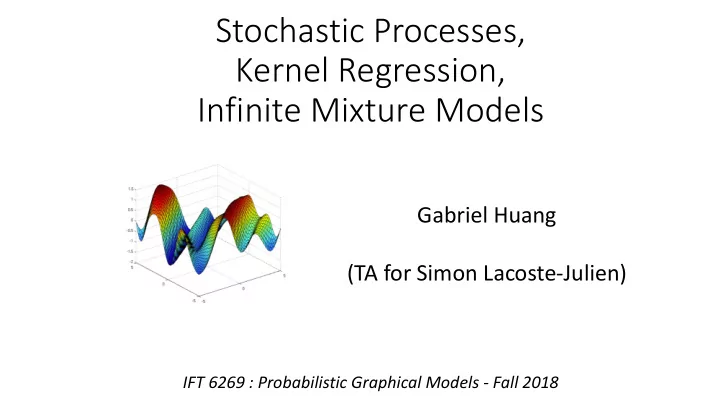
Stochastic Processes, Kernel Regression, Infinite Mixture Models Gabriel Huang (TA for Simon Lacoste-Julien) IFT 6269 : Probabilistic Graphical Models - Fall 2018

Stochastic Process = Random Function 2

Today • Motivate Gaussian and Dirichlet distribution in Bayesian Framework. • Kolmogorov’s extension theorem. • Define Gaussian Process and Dirichlet Process from finite-dimensional marginals. • Gaussian Process: • Motivating Applications: Kriging, Hyperparameter optimization. • Properties: Conditioning/Posterior distribution. • Demo. • Dirichlet Process: • Motivating Application: Clustering with unknown number of clusters. • Construction: stick-breaking, Polya urn, Chinese Restaurant Process. • De Finetti theorem. • How to use. • Demo. 3

Disclaimer I will be skipping the more theoretical building blocks of stochastic processes (e.g. measure theory) in order to be able to cover more material. 4

Recall some distributions Gaussian Distribution Samples ! in " # . Dirichlet Distribution Samples $ in Simplex Δ #&' verifies $ ' + ⋯ + $ # = 1

Why Gaussian and Dirichlet? They are often used as priors 6

Bayesians like to use those distributions as priors over model parameters !(#) Why? 7

Because they are very convenient to represent/update. Conjugate Priors 8

! "|$ ∝ ! $ " !(") Posterior Likelihood Prior model Conjugate Prior means: Posterior in same family as prior 9

! "|$ ∝ ! $ " !(") Prior Posterior "|$ ∼ )*+,,-*.(/, 1) "|$ ∼ )*+,,-*.(/′, 1′) Likelihood $|" ∼ )*+,,-*.(;, 1 < ) )*+,,-*. is conjugate prior for )*+,,-*. likelihood model. 10

! "|$ ∝ ! $ " !(") Prior Posterior "|$ ∼ )*+*,-./0(1) "|$ ∼ )*+*,-./0(1 2 ) Likelihood $|" ∼ ;<0/=>+*,<.(?) )*+*,-./0 is conjugate prior for ;<0/=>+*,<./AB.0*C>B..* likelihood model. 11

So taking the posterior is simply a matter of updating the parameters of the prior. 12

Back to Gaussian and Dirichlet Gaussian Distribution Samples ! in " # . Dirichlet Distribution Samples $ in Simplex Δ #&' verifies $ ' + ⋯ + $ # = 1

Gaussian and Dirichlet are indexed with a finite set of integers {1, … , %} . They are random vectors . (( ) , ( * , … , ( + ) (- ) , - * , … , - + ) 14

Can we index random variables with infinite sets as well? In other words, define random functions . 15

Defining stochastic processes from their marginals. 16

Suppose we want to define a random function (stochastic process) !: # ∈ % → ' , where % is an infinite set of indices. Imagine a joint distribution over all the () * ) . 17

Kolmogorov Extension Theorem informal statement Assume that for any ! ≥ 1 , and every finite subset of indices (% & , % ( , … , % * ) , we can define a marginal probability (finite-dimensional distribution) , - . ,- / ,…,- 0 (1 - . , 1 - / , … , 1 - 0 ) Then, if all marginal probabilities agree, there exists a unique stochastic process 2: % ∈ 5 → 7 which satisfies the given marginals. 18

So Kolmogorov’s extension theorem gives us a way to implicitly define stochastic processes. (However it does not tell us how to construct them.) 19

Defining Gaussian Process from finite-dimensional marginals. 20

Characterizing Gaussian Process Samples ! ∼ #$(&, () of a Gaussian Process are random functions *: , → . defined on the domain , (such as time , = . , or vectors , = . 0 ). We can also see them as an infinite collection * 1 1∈3 indexed by , . Parameters are the Mean function &(4) and Covariance function ((4, 4′) . 21

For any ! " , ! $ , … , ! & ∈ ( we define the following finite-dimensional distributions p * + , , * + - , … , * + . . * + , , * + - , … , * + . ∼ 1( 3(4 5 5 , 6 4 5 , 4 7 5,7 ) Since they are consistent with each other, Kolmogorov’s extension theorem states that they define a unique stochastic process, we will call Gaussian Process: 9 ∼ :;(3, 6) 22

Characterizing Gaussian Process Some properties are immediate consequences of definition: • ! " # = %(') 2 " # 1 − % ' - ] = Σ(', ' - ) • )*+ " # , " #- = .[ " # − % ' • Any linear combination of distinct dimensions is still a Gaussian: 9 5 : 6 ∗ " # < ∼ >(⋅,⋅) 678 23

Characterizing Gaussian Process Some properties are immediate consequences of definition: • Stationarity: Σ ", " $ = Σ " − " $ does not depend on the positions • Continuity: lim * + →* - ", "′ = - ", " • Any linear combination is still a Gaussian: 3 / 4 0 ∗ 6 7 8 ∼ :(⋅,⋅) 012 24

Example Samples 25

Posteriors of Gaussian Process. How to use them for regression? 26

Interactive Demo need a volunteer http://chifeng.scripts.mit.edu/stuff/gp-demo/ 27

Gaussian processes are very useful for doing regression on an unknown function ! : " = !(%) . Say we don’t know anything about that function, except the fact that it is smooth. 28

Before observing any data, we represent our belief on the unknown function f with the following prior: ! ∼ #$(&('), Σ(x, x , )) 7 454 6 For instance & ' = 0 and Σ ', ' , = / ⋅ exp(− ) 8 7 Controls uncertainty WARNING: Change of notation! Controls smoothness (bandwidth/length-scale) ' is now the index and !(') is the random function 29

Now, assume we observe a training set ! " = $ % , $ ' , … , $ " , ) " = ) % , ) ' , … , ) " and we want to predict the value ) ∗ = +($ ∗ ) associated with a new test point $ ∗ . One way to do that is to compute the posterior +|! " , ) " after observing the evidence (training set). 30

Bayes’ Rule + , - . , 0 . ∝ +(0 . |,, - . ) +(,) Gaussian Process Prior : • 5 6 = 89 : ; , Σ x, x > Gaussian Likelihood : • 5 ? @ 6, A @ = B(6 A , C D E @ ) -> Gaussian Process Posterior : • 5 6|A @ , ? @ = 89 :′ ; , Σ′ x, x > for some :′(;), Σ′(;, ; > ) . Remember: Gaussian Process is conjugate prior for Gaussian likelihood model. 31

Bayes’ Rule + , - . , 0 . ∝ +(0 . |,, - . ) +(,) Gaussian Process Prior : • 5 6 = 89 : ; , Σ x, x > Dirac Likelihood : ( ? → 0 ) • 5 B C 6, D C = E B C − 6 D C that is, B C is now deterministic after observing 6, D C . B C = 6 D C -> Gaussian Process Posterior : • 5 6|D C , B C = 89 :′ ; , Σ′ x, x > for some :′(;), Σ′(;, ; > ) . 32

The problem is there is no easy way to represent the parameters of the posterior ! " , Σ(", " & ) efficiently. Instead of computing the full posterior ( , we will just evaluate the posterior at one point ) ∗ = ((" ∗ ) . We want: , - ∗ . / , - / , 0 ∗ 33

We want: ! " ∗ $ % , " % , ' ∗ The finite-dimensional marginals of the Gaussian process give that: " % | $ % ∼ *( , ) ,($ % ) .($ % , ' ∗ ) .($ % , $ % ) " ∗ ' ∗ ,(' ∗ ) .(' ∗ , $ % ) .(' ∗ , ' ∗ )

Theorem: For a Gaussian vector with distribution ! $ ) * , *,* , *,+ ∼ &( , ) ) + ! " , +,* , +,+ the conditional distribution ! " |! $ is given by | ∼ &( , ) ! " /* (0 * − ) * ) ! $ ) + + , +,* , *,* /* , *,+ , +,+ − , +,* , *,* This Theorem will be useful for the Kalman filter, later on … [Schur’s complement] 35

Applying the previous theorem gives us the posterior ! ∗ . , - = ,(+ ∗ ) + 1(+ ∗ , * ) )1 * ) , * ) 23 (* ) − , * ) ) ( ) | ) ∼ %( , ( ∗ , - 1 * ) + ∗ 1 - = 1 + ∗ , + ∗ − 1(+ ∗ , * ) )1 * ) , * ) 23 1(* ) , + ∗ )

Active Learning with Gaussian Process. 37

Active Learning Active Learning is iterative process: • Generate a question ! ∗ . • Query the world with the question (by acting, can be costly) • Obtain an answer # ∗ = %(! ∗ ) . • Improve model by learning from the answer. • Repeat. 38

Active Learning Gaussian process is good for cases where it is expensive to evaluate ! ∗ = $ % ∗ . • Kriging . ! ∗ is the amount of natural resource, % ∗ is new 2D/3D location to dig. Every evaluation is mining and can cost millions. • Hyperparameter optimization (Bayesian optimization). ! ∗ is the validation loss, % ∗ is set of hyperparameters to test. Every evaluation is running an experiment and can take hours. 39

Back to the demo (Talk about utility function) http://chifeng.scripts.mit.edu/stuff/gp-demo/ 40

Formal equivalence with Kernelized Linear Regression. [blackboard if time] Rasmussen & Williams (2006) http://www.gaussianprocess.org/gpml/chapters/RW2.pdf 41

Dirichlet Processes. Stick Breaking Construction 42

) = () & , ) / , … ) ∼ !78(9) - & , - / , … ∼ 223 ! 4 scalar weights parameters, sampled sum up to 1 from base distribution '( ! = # ) $ * + , Diracs concentrate $%& probability mass ) $ at - $ G is a random probability measure : • random : both ) and - are random • probability measure : it is a convex combination of Diracs, which are probability measures 43

Courtesy of Khalid El-Arini 44