STIS First-Order Low-Resolution Mode Point-Source Sensitivity Curves - PDF document

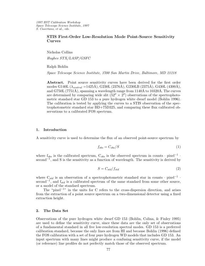
1997 HST Calibration Workshop Space Telescope Science Institute, 1997 S. Casertano, et al., eds. STIS First-Order Low-Resolution Mode Point-Source Sensitivity Curves Nicholas Collins Hughes STX/LASP/GSFC Ralph Bohlin Space Telescope Science Institute, 3700 San Martin Drive, Baltimore, MD 21218 Point source sensitivity curves have been derived for the first order Abstract. modes G140L ( λ central =1425˚ A), G230L (2376˚ A), G230LB (2375˚ A), G430L (4300˚ A), and G750L (7751˚ A), spanning a wavelength range from 1140˚ A to 10320˚ A. The curves are determined by comparing wide slit (52 ′′ × 2 ′′ ) observations of the spectrophoto- metric standard star GD 153 to a pure hydrogen white dwarf model (Bohlin 1996). The calibration is tested by applying the curves to a STIS observation of the spec- trophotometric standard star BD+75D325, and comparing these flux calibrated ob- servations to a calibrated FOS spectrum. 1. Introduction A sensitivity curve is used to determine the flux of an observed point-source spectrum by f obs = C obs /S (1) where f obs is the calibrated spectrum, C obs is the observed spectrum in counts · pixel − 1 · second − 1 , and S is the sensitivity as a function of wavelength. The sensitivity is derived by S = C std /f std (2) where C std is an observation of a spectrophotometric standard star in counts · pixel − 1 · second − 1 , and f std is a calibrated spectrum of the same standard from some other source, or a model of the standard spectrum. The “pixel − 1 ” in the units for C refers to the cross-dispersion direction, and arises from the extraction of a point source spectrum on a two-dimensional detector using a fixed extraction height. 2. The Data Set Observations of the pure hydrogen white dwarf GD 153 (Bohlin, Colina, & Finley 1995) are used to define the sensitivity curve, since these data are the only set of observations of a fundamental standard in all five low-resolution spectral modes. GD 153 is a preferred calibration standard, because the only lines are from HI and because Bohlin (1996) defined the FOS calibration with a set of four pure hydrogen WD models that includes GD 153. An input spectrum with many lines might produce a confusing sensitivity curve, if the model (or reference) line profiles do not perfectly match those of the observed spectrum. 77

78 Collins & Bohlin 2.1. Observations All input spectra were obtained using the clear aperture # 38 (52 ′′ × 2 ′′ ). Two averaged observations comprise the input spectrum for the far-UV MAMA mode G140L. Only one near-UV (G230L) observation of GD 153 was obtained through aperture # 38. For each of the three CCD modes (G230LB, G430L, and G750L), seven observations were averaged to produce high signal to noise spectra. The component spectra that make up the average spectrum for each mode are listed in Table 1. Table 1. Observations Rootname Observation Target Optical CRSPLIT Total Slit Slit Date Element ExpTime Number Size (”) (sec.) O43J01QAM 09/07/97 GD153 G140L 0 60.0 38 52x2 O3ZX08HHM 13/07/97 GD153 G140L 0 187.0 38 52x2 O3ZX08HLM 13/07/97 GD153 G230L 0 187.1 38 52x2 O3TT42010 21/05/97 GD153 G230LB 2 600.0 38 52x2 O3TT43010 28/05/97 GD153 G230LB 2 600.0 38 52x2 O3TT44010 04/06/97 GD153 G230LB 2 600.0 38 52x2 O3TT45010 10/06/97 GD153 G230LB 2 600.0 38 52x2 O3TT46010 18/06/97 GD153 G230LB 2 600.0 38 52x2 O3TT47010 25/06/97 GD153 G230LB 2 600.0 38 52x2 O3TT48010 01/07/97 GD153 G230LB 2 600.0 38 52x2 O3TT42020 21/05/97 GD153 G430L 2 252.0 38 52x2 O3TT43020 28/05/97 GD153 G430L 2 252.0 38 52x2 O3TT44020 04/06/97 GD153 G430L 2 252.0 38 52x2 O3TT45020 10/06/97 GD153 G430L 2 252.0 38 52x2 O3TT46020 18/06/97 GD153 G430L 2 252.0 38 52x2 O3TT47020 25/06/97 GD153 G430L 2 252.0 38 52x2 O3TT48020 01/07/97 GD153 G430L 2 252.0 38 52x2 O3TT42040 21/05/97 GD153 G750L 2 3240.0 38 52x2 O3TT43040 28/05/97 GD153 G750L 2 3240.0 38 52x2 O3TT44040 04/06/97 GD153 G750L 2 3240.0 38 52x2 O3TT45040 10/06/97 GD153 G750L 2 3240.0 38 52x2 O3TT46040 18/06/97 GD153 G750L 2 2282.0 38 52x2 O3TT47040 25/06/97 GD153 G750L 2 2282.0 38 52x2 O3TT48040 01/07/97 GD153 G750L 2 2282.0 38 52x2 The spectral extraction heights for the component spectra are 11 pixels for G140L and G230L, and 7 pixels for G230LB, G430L, and G750L (Leitherer & Bohlin 1997). Each of the seven component G750L spectra was fringe-corrected at long wavelengths using a library tungsten lamp flat before averaging them together. For this data set, all tungsten lamp flats used were obtained through slit # 35 (52 ′′ × 0 . ′′ 1). Briefly, the library flats are generated by (Plait, 1997) • removing the lamp spectrum from the flat, • removing scattered light (as determined by profiles obtained along the fiducial bars in the dispersion direction), Profiles of the data and library flat are cross-correlated to ensure that the fringes in both are in phase. If the fringes are not in phase, the library flat is shifted (typically less than 1 pixel) to match the phase of the fringes in the data. The shifted library flat is then applied to the data image. 2.2. Reference Spectrum The reference spectrum, GD153 MOD 002, is a pure hydrogen white dwarf model normal- ized to Landolt’s visual photometry (Bohlin 1996). The spectrum was obtained from the

79 STIS Sensitivity Curves Calibration Data Base System (CDBS) at http://www.stsci.edu/ftp/instrument/news/ Observatory/astronomical_catalogs.html . 3. Data Reduction For each optical mode, the reference spectrum is integrated to match the resolution of each co-added observation, then divided into the observed spectrum, yielding a sensitivity curve in units of counts · pixel − 1 · second − 1 ergs · second − 1 · cm − 2 · ˚ A − 1 A spline fit with evenly spaced nodes is performed to each raw curve in order to obtain a smooth sensitivity curve. Each fit is refined by interactively selecting more nodes in regions where a curve varies greatly with small changes in wavelength. Table 2 lists the number of nodes used within the nominal wavelength range for each mode. The wavelength region 1200˚ A - 1225˚ A in mode G140L is masked to exclude the strong Ly α feature from the fit. Small residuals at the Balmer lines on G430L and G750L are caused by slight differences in resolution between STIS and the model spectrum. Some of the sensitivity curve spline fits are extrapolated at either end by at most 20 pixels to account for future planned spectral format, or MSM, shifts. No extrapolation is done past very low signal-to-noise regions. Some curves are cut off in low signal-to-noise regions. Table 2 lists the extrapolated and cropped regions for each mode. Table 2. Sensitivity Curve Extrapolation Regions Optical Spline Nominal Short- λ Long- λ Short- λ Full Range(˚ Extrap.(˚ Extrap.(˚ Cutoff (˚ Range (˚ Element Nodes A) A) A) A) A) 1140˚ G140L 26 1118 - 1713 no extrap. 1713 - 1724 A 1140 - 1724 1600˚ G230L 28 1563 - 3140 no extrap. 3140 - 3171 A 1600 - 3171 G230LB 28 1664 - 3066 1650 - 1664 3066 - 3093 - 1650 - 3093 G430L 40 2885 - 5691 2881 - 2884 5691 - 5746 - 2881 - 5746 G750L 42 5235 - 10229 no extrap. 10229 - 10327 - 5235 - 10327 4. Results The sensitivity curves and their residuals are shown in Figures 1–5. The spline fit and extrapolations described above are represented by the dashed line in each plot. The spline nodes are plotted with diamonds. 4.1. Error Analysis The residuals shown in Figures 1–5 are determined by dividing each curve by its spline fit, and are plotted for the wavelength ranges listed in Table 3. Table 3 lists the percent root-mean-squared residuals averaged over all wavelengths for each mode. Average RMS residuals are listed for three wavelength ranges for mode G750L to show how the scatter increases in the long wavelength region subject to fringing.