Steady-State Simulation Reading: Ch. 9 in Law & Ch. 15 in - PowerPoint PPT Presentation

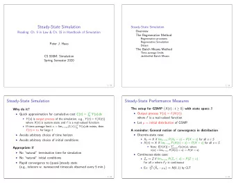
Steady-State Simulation Reading: Ch. 9 in Law & Ch. 15 in Handbook of Simulation Peter J. Haas CS 590M: Simulation Spring Semester 2020 1 / 34

Steady-State Simulation Overview The Regenerative Method Regenerative processes Regenerative Simulation Delays The Batch Means Method Time-average limits Jackknifed Batch Means 2 / 34

Steady-State Simulation Why do it? R t I Quick approximation for cumulative cost C ( t ) = 0 Y ( s ) ds I Y ( s ) is output process of the simulation, e.g., Y ( t ) = f � � X ( t ) where X ( t ) is system state and f is a real-valued function R t I If time-average limit α = lim t !1 (1 / t ) 0 Y ( s ) ds exists, then C ( t ) ⇡ t α for large t I Avoids arbitrary choice of time horizon I Avoids arbitrary choice of initial conditions Appropriate if I No “natural” termination time for simulation I No “natural” initial conditions I Rapid convergence to (quasi-)steady state (e.g., telecom w. nanosecond timescale observed every 5 min.) 3 / 34

Steady-State Performance Measures � � The setup for GSMP X ( t ) : t � 0 with state space S I Output process Y ( t ) = f � � X ( t ) where f is a real-valued function I Let µ = initial distribution of GSMP A reminder: General notion of convergence in distribution I Discrete-state case: I X n ) X if lim n !1 P ( X n = s ) = P ( X = s ) for all s 2 S discrete time - I X ( t ) ) X if lim t !1 P � � X ( t ) = s = P ( X = s ) for all s 2 S cent . time - I Note: E [ f ( X )] = P s ∈ S f ( s ) π ( s ), where � � π ( s ) = lim t →∞ P X ( t ) = s = P ( X = s ) I Continuous-state case: I Z n ) Z if lim n !1 P ( Z n  x ) = P ( Z  x ) for all x where F Z is continuous � ¯ p n I Ex: X n � µ X � ) N (0 , 1) by CLT σ 4 / 34

Steady-State Performance Measures, Continued Time-Average Limit of Y ( t ) process R t n o α such that P µ lim t !1 (1 / t ) 0 Y ( u ) du = α = 1 for any µ Steady-State Mean of Y ( t ) process α = E [ f ( X )], where, for any µ , X ( t ) ) X and E [ f ( X )] exists Limiting Mean of Y ( t ) process ⇥ � �⇤ α = lim t !1 E f X ( t ) for any µ I “for any µ ” = for any member of GSMP family indexed by µ (with other building blocks the same) I E [ f ( X )] exists if and only if E [ | f ( X ) | ] < 1 I If f is bounded or S is finite, then X ( t ) ) X implies ⇥ � �⇤ lim t !1 E f X ( t ) = E [ f ( X )] (s-s mean = limiting mean) 5 / 34

Steady-State Simulation Challenges Autocorrelation problem I For time-average limit, R t α = lim t !1 ¯ Y ( t ) = lim t !1 (1 / t ) 0 Y ( u ) du I Natural estimator of α is ¯ Y ( t ) for some large t (obtained from one long observation of system) I But Y ( t ) and Y ( t + ∆ t ) highly correlated if ∆ t is small I So estimator is average of autocorrelated observations I Techniques based on i.i.d. observations don’t work Initial-Transient Problem I Steady-state distribution unknown, so initial dist’n is not typical of steady-state behavior I Autocorrelation implies that initial bias will persist I Very hard to detect “end of initial-transient period” 6 / 34

Estimation Methods Many alternative estimation methods I Regenerative method I Batch-means method I Autoregressive method I Standardized-time-series methods I Integrated-path method I . . . We will focus on: I Regenerative method: clean and elegant I Batch means: simple, widely used and the basis for other methods 7 / 34

Steady-State Simulation Overview The Regenerative Method Regenerative processes Regenerative Simulation Delays The Batch Means Method Time-average limits Jackknifed Batch Means 8 / 34

The Regenerative Method References: I Shedler [Ch. 2 & 3], Haas [Ch. 5 & 6] I Recent developments: ACM TOMACS 25(4), 2015 Regenerative Processes I Intuitively: � � X ( t ) : t � 0 is regenerative if process “probabilistically restarts” infinitely often I Restart times T (0) , T (1) , . . . called regeneration times or regeneration points en I Regeneration points are random I Must be almost surely (a.s.) finite I Ex: Arrivals to empty GI/G/1 queue queue 9 / 34

Regenerative Processes: Formal Definition Definition: Stopping time A random variable T is a stopping time with respect to � � X ( t ) : t � 0 if occurrence or non-occurrence of event { T  t } is � � completely determined by X ( u ) : 0  u  t Definition: Regenerative process � � The process X ( t ) : t � 0 is regenerative if there exists an infinite � � sequence of a.s. finite stopping times T ( k ) : k � 0 s.t. for k � 1 � � � � X ( t ) : t � T ( k ) X ( t ) : t � T (0) 1. is distributed as � � � � 2. X ( t ) : t � T ( k ) is independent of X ( t ) : t < T ( k ) I If T (0) = 0, process is non-delayed (else delayed) I Can drop stopping-time requirement, (more complicated def.) I � � � � X ( t ) : t � 0 regen. ) : t � 0 f X ( t ) regen. I Analogous definition for discrete-time processes 10 / 34

Regenerative Processes: Examples Ex 1: Successive times that CTMC hits a fixed state x start in state x ) ( I Formally, T (0) = 0 and T ( k ) = min { t > T ( k � 1) : X ( t � ) 6 = x and X ( t ) = x } I Observe that X � � T ( k ) = x for all k I The two regenerative criteria follow from Markov property Ex 2: Successive times that CTMC leaves a fixed state x I X � � T ( k ) distributed according to P ( x , · ) for each k I Second criterion follows from Markov property . fees Q: Is a semi-Markov process regenerative? definitions above examples In as same because of Markov property at " transition times state 11 / 34

Regenerative GSMPs Ex 3: GSMP with a single state I ¯ s 2 S is a single state if E (¯ s ) = { ¯ e } for some ¯ e 2 E I Regeneration points: successive times that ¯ e occurs in ¯ s I Observe that for each k � 1, I New state s 0 at T ( k ) distributed according to p ( · ; ¯ s , ¯ e ) I No old clocks I Clock for new event e 0 distributed as F ( · ; s 0 , e 0 , ¯ s , ¯ e ) I Regenerative property follows from Markov property for � � ( S n , C n ) : n � 0 ( In - Markov process a semi a single state ) , every state is Ex 4: GI/G/1 queue I X ( t ) = number of jobs in system at time t I � � X ( t ) : t � 0 is a GSMP I T ( k ) = time of k th arrival to empty system (why?) a single - state ⑥ is because 12 / 34

Regenerative GSMPs, Continued Ex 5: Cancellation I Suppose there exist ¯ s 0 , ¯ s 2 S and ¯ e 2 E (¯ s ) with e ) = ; p (¯ s 0 ; ¯ s , ¯ e ) r (¯ s , ¯ e ) > 0 such that O (¯ s 0 ; ¯ s , ¯ I T ( k ) = k th time that ¯ e occurs in ¯ s and new state is ¯ s 0 new state chosen according to Ex 6: Exponential clocks I Suppose that . ; sie ) pc I There exists ˜ E ✓ E such that each e 2 ˜ E is a simple event with F ( x ; e ) = 1 � e � λ ( e ) x e } ✓ ˜ I There exists ¯ s 2 S and ¯ e 2 E (¯ s ) s.t. E (¯ s ) � { ¯ E I T ( k ) = k th time that ¯ e occurs in ¯ s (memoryless property) old clock reading ton ee E is n exp likes ) Other (fancier) regeneration point constructions are possible I E.g., if clock-setting distn’s have heavier-than-exponential � 1 � F ( t ) � tails or bounded hazard rates h ( t ) = f ( t ) / 13 / 34

Steady-State Simulation Overview The Regenerative Method Regenerative processes Regenerative Simulation Delays The Batch Means Method Time-average limits Jackknifed Batch Means 14 / 34

Regenerative Simulation: Cycles Regeneration points decompose process into i.i.d. cycles � � I k th cycle: X ( t ) : T ( k � 1)  t < T ( k ) I Length of k th cycle: τ k = T ( k ) � T ( k � 1) R T ( k ) I Set Y k = T ( k � 1) Y ( u ) du I The pairs ( Y 1 , τ 1 ) , ( Y 2 , τ 2 ) , . . . are i.i.d as ( Y , τ ) Initial transient is not a problem! 15 / 34

Regenerative Simulation: Time-Average Limits R t I Recall: ¯ Y ( t ) = (1 / t ) 0 Y ( u ) du Theorem Suppose that E [ | Y 1 | ] < 1 and E [ τ 1 ] < 1 . Then lim t !1 ¯ Y ( t ) = α a.s., where α = E [ Y ] / E [ τ ]. I So estimating time-average limit reduces to a ratio-estimation problem (can use delta method, jackknife, bootstrap) (Most of) Proof R T ( j ) P n Z T ( n ) P n T ( j � 1) Y ( u ) du j =1 Y j 1 j =1 ¯ � � � = Y T ( n ) = Y ( u ) du = P n P n � T ( n ) T ( j ) � T ( j � 1) j =1 τ j 0 j =1 ¯ � � ) lim T ( n ) = α a.s. by SLLN Y n !1 16 / 34

Regenerative Simulation: Steady-State Means Definition A real-valued random variable τ is said to be periodic with period d if d is the largest real number such that, w.p.1, τ assumes values in the set { 0 , d , 2 d , 3 d , . . . } . If no such number exists, then τ is aperiodic. (A discrete random variable is aperiodic if d = 1.) Theorem � � Suppose that X ( t ) : t � 0 is regenerative with finite state space S and τ is aperiodic with E [ τ ] < 1 . Then X ( t ) ) X and E [ f ( X )] = E [ Y 1 ( f )] / E [ τ 1 ] for any real-valued function f on S , R T (1) � � where Y 1 ( f ) = T (0) f X ( u ) du and τ 1 = T (1) � T (0) I Under conditions of theorem, time avg limit is also a steady-state mean (and a limiting mean) ;yELP(xaD ] . limit : gli time avg 17 / 34