Statistics and learning Analysis of variance (ANOVA) Emmanuel - PowerPoint PPT Presentation
Statistics and learning Analysis of variance (ANOVA) Emmanuel Rachelson and Matthieu Vignes ISAE SupAero Friday 25 th January 2013 E. Rachelson & M. Vignes (ISAE) SAD 2013 1 / 10 ANOVA: presentation Allows to evaluate and compare the
Statistics and learning Analysis of variance (ANOVA) Emmanuel Rachelson and Matthieu Vignes ISAE SupAero Friday 25 th January 2013 E. Rachelson & M. Vignes (ISAE) SAD 2013 1 / 10
ANOVA: presentation ◮ Allows to evaluate and compare the effect of one or several controlled factors on a population from the point of view of a given variable. ◮ Under the hypothesis of Gaussian distribution, ANOVA is just a global test to compare the means of subpopulations associated to the levels of the considered factors. E. Rachelson & M. Vignes (ISAE) SAD 2013 2 / 10
1 way-ANOVA ◮ a factor can take k different values. To each level is associated X i ∼ N ( µ i , σ 2 ) . ◮ µ i ’s are unknown, σ is known. ◮ ∀ 1 ≤ i ≤ k , a sample of size n i is taken from subpopulation i (we write n = � n i ): ( X 1 i = x 1 i , . . . , X n i = x n i i ) i E. Rachelson & M. Vignes (ISAE) SAD 2013 3 / 10
1 way-ANOVA ◮ a factor can take k different values. To each level is associated X i ∼ N ( µ i , σ 2 ) . ◮ µ i ’s are unknown, σ is known. ◮ ∀ 1 ≤ i ≤ k , a sample of size n i is taken from subpopulation i (we write n = � n i ): ( X 1 i = x 1 i , . . . , X n i = x n i i ) i ◮ Finally the ANOVA is a test: ANOVA = test of equality for all means (H0) m 1 = m 2 = . . . = m k and (H1) ∃ p, q such that m p � = m q E. Rachelson & M. Vignes (ISAE) SAD 2013 3 / 10
1 way-ANOVA explained ◮ Variable X j i associated to the j th draw can be decomposed into X j i = µ + α i + ǫ j i , ◮ where µ is the mean of all X , α i is the mean effect due to level i of the considered factor and ǫ is the residual, with N (0 , σ 2 ) distribution. ◮ Note that µ + α i is the mean of X on population i which corresponds to level i of the factor. � ni j =1 X j j X j � k � ◮ Some notations: ¯ , ¯ X = i =1 i X i = i and more n n i specifically: X ) 2 (variance between), A = 1 i n i ( ¯ X i − ¯ ◮ S 2 � n X i ) 2 (residual variance) and j ( X j i − ¯ S 2 R = 1 � � i n X ) 2 (total variance) j ( X j i − ¯ S = 1 � � n i E. Rachelson & M. Vignes (ISAE) SAD 2013 4 / 10
1 way-ANOVA: theory Theorem (1 way-ANOVA formula) S 2 = S 2 A + S 2 R Theorem (Useful ”cooking recipe” for the test) R /σ 2 ∼ χ 2 ( n − k ) . 1. nS 2 2. Under (H0), nS 2 /σ 2 ∼ χ 2 ( n − 1) and nS 2 A /σ 2 ∼ χ 2 ( k − 1) . So that under (H0), S 2 A / ( k − 1) R / ( n − k ) ∼ F ( k − 1; n − k ) , a Fisher Snedecor S 2 distribution with ( k − 1; n − k ) dof. Morality: we just test whether S 2 A is small compared to S 2 R : is the between dispersion small as compared to the inner dispersion ? E. Rachelson & M. Vignes (ISAE) SAD 2013 5 / 10
2 way-ANOVA ◮ We just want to generalise that to 2 factors A and B with resp. p and q levels. ◮ to the ( i, j ) couple of levels for both factors correspond a sample of size n i,j for measured variable X . ◮ The statistical model is balanced if n i,j = r, ∀ ( i, j ) . We restrict the presentation in this framework to keep notations more simple. ◮ So to any couple of levels ( i, j ) is associated sample ( X 1 i,j = x 1 i,j , . . . , X r i,j = x r i,j ) . ◮ X i,j is assumed to be N ( µ i,j , σ 2 ) and we can decompose... E. Rachelson & M. Vignes (ISAE) SAD 2013 6 / 10
2-way ANOVA decomposition ◮ µ i,j = µ + α i + β j + γ i,j , ◮ with resp. effects for A , B and the A × B interaction. � p � q � r k =1 X k ◮ We adapt previous notations: ¯ i =1 j =1 i,j X = , pqr k X k k X k k X k � � � � � ¯ ¯ ¯ X i,j = i,j , X i, • = j i,j and X • ,j = i i,j and for r qr pr variances: ◮ S 2 x ) 2 , S 2 x ) 2 , A = qr � i ( ¯ x i, • − ¯ B = pr � j ( ¯ x • ,j − ¯ S 2 x ) 2 , AB = r � � j ( ¯ x i,j − ¯ x i, • − ¯ x • ,j + ¯ u x i,j ) 2 and S 2 = � S 2 k ( x k k ( x k x ) 2 . i,j − ¯ i,j − ¯ R = � � � � � i j i j Whooosh ! E. Rachelson & M. Vignes (ISAE) SAD 2013 7 / 10
2 way-ANOVA: theory Theorem (Formula for 2 way ANOVA) S 2 = S 2 A + S 2 B + S 2 AB + S 2 R Proof is tedious and does not have that much interest. Instead of listing all distributions, we summarise all of that in the table on the next slide... E. Rachelson & M. Vignes (ISAE) SAD 2013 8 / 10
2 way-ANOVA analysis table Variat. origin � ( squares ) d.o.f. Mean squares F-variable S 2 S 2 A / ( p − 1) = S 2 S 2 Am /S 2 A p − 1 A Am Rm S 2 S 2 B / ( q − 1) = S 2 S 2 Bm /S 2 B q − 1 B Bm Rm S 2 S 2 ( p − 1)( q − 1) = S 2 S 2 ABm /S 2 A × B ( p − 1)( q − 1) AB AB ABm Rm S 2 S 2 R / ( p − 1) = S 2 Residual pq ( r − 1) R Rm S 2 Total pqr − 1 E. Rachelson & M. Vignes (ISAE) SAD 2013 9 / 10
That’s all For today: next week → regression !! E. Rachelson & M. Vignes (ISAE) SAD 2013 10 / 10
Recommend
More recommend
Explore More Topics
Stay informed with curated content and fresh updates.
