Multivariate Analysis of Variance Max Turgeon STAT 4690Applied - PowerPoint PPT Presentation
Multivariate Analysis of Variance Max Turgeon STAT 4690Applied Multivariate Analysis Quick Overview What do we mean by Analysis of Variance? ANOVA is a collection of statistical models that aim to analyze and understand the difgerences
Multivariate Analysis of Variance Max Turgeon STAT 4690–Applied Multivariate Analysis
Quick Overview What do we mean by Analysis of Variance? • ANOVA is a collection of statistical models that aim to analyze and understand the difgerences in means between difgerent subgroups of the data. • Note that there could be multiple, overlapping ways of defjning the subgroups (e.g multiway ANOVA) • It also provides a framework for hypothesis testing. • Which can be recovered from a suitable regression model. • Most importantly , ANOVA provides a framework for understanding and comparing the various sources of variation in the data. 2 • As such, it can be seen as a generalisation of the t -test (or of Hotelling’s T 2 ).
Review of univariate ANOVA i ... • We are interested in testing the hypothesis that • Homoscedasticity . . . . . . 3 • Assume the data comes from g populations: X 11 , . . . , X 1 n 1 X g 1 , . . . , X gn g • Assume that X ℓ 1 , . . . , X ℓn ℓ is a random sample from N ( µ ℓ , σ 2 ) , for ℓ = 1 , . . . , g . µ 1 = . . . = µ g .
Review of univariate ANOVA ii • We can write our observations as otherwise there are infjnitely many models that lead to the same data-generating mechanism. 4 • Reparametrisation : We will write the mean µ ℓ = µ + τ ℓ as a sum of an overall component µ (i.e. shared by all populations) and a population-specifjc component τ ℓ . • Our hypothesis can now be rewritten as τ ℓ = 0 , for all ℓ . X ℓi = µ + τ ℓ + ε ℓi , where ε ℓi ∼ N (0 , σ 2 ) . • Identifjability : We need to assume ∑ g ℓ =1 τ ℓ = 0 ,
Review of univariate ANOVA iii • We get the following decomposition: 5 ∑ g • Sample statistics : Set n = ℓ =1 n ℓ . • Overall sample mean: ¯ ∑ g ∑ n ℓ X = 1 i =1 X ℓi . n ℓ =1 • Population-specifjc sample mean: ¯ 1 ∑ n ℓ X ℓ = i =1 X ℓi . n ℓ ( ¯ ( X ℓi − ¯ ) X ℓ − ¯ ) ( X ℓi − ¯ ) X = X + X ℓ . • Squaring the left-hand side and summing over both ℓ and i , we get ( ¯ g n ℓ g g n ℓ ) 2 = ) 2 . ) 2 + X ℓi − ¯ X ℓ − ¯ X ℓi − ¯ ( ( ∑ ∑ ∑ ∑ ∑ X n ℓ X X ℓ i =1 i =1 ℓ =1 ℓ =1 ℓ =1
Review of univariate ANOVA iv • The model (or treatment) sum of squares : • The residual sum of squares : 6 • The total sum of squares : • This is typically summarised as SS T = SS M + SS R : ) 2 ( SS T = ∑ g ∑ n ℓ X ℓi − ¯ X ℓ =1 i =1 ( ¯ ) 2 SS M = ∑ g X ℓ − ¯ ℓ =1 n ℓ X ) 2 SS R = ∑ g ∑ n ℓ ( X ℓi − ¯ X ℓ ℓ =1 i =1
Review of univariate ANOVA v Residual Total • Yet another representation is the ANOVA table : 7 Model Degrees of freedom Sum of Squares Source of Variation SS M g − 1 SS R n − g SS T n − 1 • The usual test statistic used for testing τ ℓ = 0 for all ℓ is F = SS M / ( g − 1) SS R / ( n − g ) ∼ F ( g − 1 , n − g ) .
Review of univariate ANOVA vi • We could also instead reject the null hypothesis for small values of This is the test statistic that we will generalize to the multivariate setting. 8 SS R = SS R . SS R + SS M SS T
Multivariate ANOVA i . • We are again interested in testing the hypothesis that • Homoscedasticity is key here again. . . ... . . . populations: 9 • The setting is similar: Assume the data comes from g Y 11 , . . . , Y 1 n 1 Y g 1 , . . . , Y gn g • Assume that Y ℓ 1 , . . . , Y ℓn ℓ is a random sample from N p ( µ ℓ , Σ) , for ℓ = 1 , . . . , g . µ 1 = . . . = µ g .
Multivariate ANOVA ii • Instead of a decomposition of the sum of squares, we get a decomposition of the outer product: 10 • Reparametrisation : We will write the mean as µ ℓ = µ + τ ℓ • Y ℓi = µ + τ ℓ + E ℓi , where E ℓi ∼ N p (0 , Σ) . • Identifjability : We need to assume ∑ g ℓ =1 τ ℓ = 0 . ( Y ℓi − ¯ Y )( Y ℓi − ¯ Y ) T .
Multivariate ANOVA iii • The decomposition is given as • Within sum of squares and cross products matrix : • Between sum of squares and cross products matrix : 11 g n ℓ g Y ) T = ∑ ∑ ( Y ℓi − ¯ Y )( Y ℓi − ¯ ∑ n ℓ ( ¯ Y ℓ − ¯ Y )( ¯ Y ℓ − ¯ Y ) T i =1 ℓ =1 ℓ =1 g n ℓ ∑ ∑ ( Y ℓi − ¯ Y ℓ )( Y ℓi − ¯ Y ℓ ) T . + ℓ =1 i =1 ∑ g ℓ =1 n ℓ ( ¯ Y ℓ − ¯ Y )( ¯ Y ℓ − ¯ Y ) T . B = ∑ g ∑ n ℓ i =1 ( Y ℓi − ¯ Y ℓ )( Y ℓi − ¯ Y ℓ ) T . W = ℓ =1
Multivariate ANOVA iv Degrees of freedom statistic: Total Residual Model 12 Sum of Squares Source of Variation ∑ g • Note that W = ℓ =1 ( n ℓ − 1) S ℓ . • Similarly as above, we have a MANOVA table : B g − 1 W n − g B + W n − 1 • To test the null hypothesis H 0 : τ ℓ = 0 for all ℓ = 1 , . . . , g , we will use Wilk’s lambda as our test | W | Λ = | B + W | .
Multivariate ANOVA v • There is actually no closed-form for the null distribution value, we reject the null hypothesis if 13 of Λ , so we will use Bartlett’s approximation: n − 1 − 1 ( ) log Λ ≈ χ 2 (( g − 1) p ) . − 2( p + g ) • In particular, if we let c = χ 2 α (( n − 1) p ) be the critical ( ) − c Λ ≤ exp . n − 1 − 0 . 5( p + g )
Example i ## Example on producing plastic film ## from Krzanowski (1998, p. 381) 6.9, 6.1, 6.3, 6.7, 6.6, 7.2, 7.1, 6.8, 7.1, 7.0, 7.2, 7.5, 7.6) 9.9, 9.5, 9.4, 9.1, 9.3, 8.3, 8.4, 8.5, 9.2, 8.8, 9.7, 10.1, 9.2) opacity <- c (4.4, 6.4, 3.0, 4.1, 0.8, 5.7, 2.0, 3.9, 1.9, 5.7, 2.8, 4.1, 3.8, 1.6, 3.4, 8.4, 5.2, 6.9, 2.7, 1.9) 14 tear <- c (6.5, 6.2, 5.8, 6.5, 6.5, 6.9, 7.2, gloss <- c (9.5, 9.9, 9.6, 9.6, 9.2, 9.1, 10.0,
Example ii Y <- cbind (tear, gloss, opacity) Y_low <- Y[1 : 10,] Y_high <- Y[11 : 20,] W <- ( nrow (Y_low) - 1) *cov (Y_low) + ( nrow (Y_high) - 1) *cov (Y_high) B <- (n-1) *cov (Y) - W ## [1] 0.4136192 15 n <- nrow (Y); p <- ncol (Y); g <- 2 (Lambda <- det (W) /det (W + B))
Example iii transf_lambda <- - (n - 1 - 0.5 * (p + g)) *log (Lambda) ## [1] TRUE # Or if you want a p-value pchisq (transf_lambda, p * (g-1), lower.tail = FALSE) ## [1] 0.002227356 16 transf_lambda > qchisq (0.95, p * (g-1))
Example iv # R has a function for MANOVA # But first, create factor variable rate <- gl (g, 10, labels = c ("Low", "High")) fit <- manova (Y ~ rate) summary_tbl <- broom ::tidy (fit, test = "Wilks") # Or you can use the summary function knitr ::kable (summary_tbl, digits = 3) 17
Example v 3 - - - - - 18 Residuals 0.002 16 7.561 term 0.414 1 rate p.value den.df num.df statistic wilks df 18
Example vi # Check residuals for evidence of normality library (tidyverse) residuals %>% as.data.frame () %>% gather (variable, residual) %>% ggplot ( aes (sample = residual)) + stat_qq () + stat_qq_line () + facet_grid (. ~ variable) + theme_minimal () 19 fit %>%
Example vii 20 gloss opacity tear 2.5 sample 0.0 −2.5 −2 −1 0 1 2 −2 −1 0 1 2 −2 −1 0 1 2 theoretical
Comments i • The output from R shows a difgerent approximation to the Wilk’s lambda distribution, due to Rao. • There are actually 4 tests available in R (we will discuss them in the next lecture): • Wilk’s lambda; • Pillai-Bartlett; • Hotelling-Lawley; • Roy’s Largest Root. 21
Comments ii • Since we only had two groups in the above example, we were only comparing two means. • Wilk’s lambda was therefore equivalent to Hotelling’s • But of course MANOVA is much more general. • We can assess the normality assumption by looking at the 22 T 2 . residuals E ℓi = Y ℓi − ¯ Y ℓ .
Testing for Equality of Covariance Matrices i • Last lecture, when comparing two multivariate means, and again today, we talked about homoscedasticity as an important assumption. • This is a testable assumption, i.e. we can devise a corresponding hypothesis test. • In this course, we will discuss Box’s M-test • This test is based on a comparison of generalized variances. 23 • Our null hypothesis: H 0 : Σ 1 = · · · = Σ g , where Σ ℓ is the covariance matrix for population ℓ .
Testing for Equality of Covariance Matrices ii • Under the normality assumption, the likelihood ratio 24 statistic for the null hypothesis above is ( | S ℓ | ) ( n ℓ − 1) / 2 g ∏ Λ = . | S pool | ℓ =1 • Here, S ℓ is the sample covariance for population ℓ , and S pool is the pooled estimator: ( g ) 1 1 ∑ S pool = ( n ℓ − 1) S ℓ = n − 1 W. n − 1 ℓ =1
Testing for Equality of Covariance Matrices iii • Box’s M-statistic is defjned as • The general theory of Likelihood Ratio Tests tells us that 25 M = − 2 log Λ . M ≈ χ 2 ( ν ) for an appropriate value ν > 0 .
Testing for Equality of Covariance Matrices iv Box’s Test for Equality of Covariance Matrices where 26 Set ) ( 2 p 2 + 3 p − 1 ( g 1 1 ) ∑ u = n ℓ − 1 − . n − g 6( p + 1)( g − 1) ℓ =1 Then C = (1 − u ) M has approximate χ 2 ( ν ) distribution, ν = 1 2 p ( p + 1)( g − 1) .
Recommend
More recommend
Explore More Topics
Stay informed with curated content and fresh updates.




![Variance = E[I 2 ] 2pE[I] + p 2 = E[I] 2p p + p 2 = 2 2 = p-2p+ p pq variance.1](https://c.sambuz.com/1069957/variance-s.webp)
